1  Introduction to Spatial Econometrics

1.1 Why Do We Need Spatial Econometrics?

An essential consideration in any study involving spatial units—such as neighborhoods, municipalities, regions, or countries—is that observations may be connected rather than independent. Economic activity, environmental processes, infrastructure, migration, trade, public policy, and social interaction frequently cross administrative boundaries. Spatial econometrics provides models and inferential methods for studying data generated in such interconnected systems.

Consider Figure 1.1, where Region 3 (R3) is highly industrialized, while Regions 1, 2, 4, and 5 are primarily residential. If economic activity increases in R3, pollution may rise not only within that region but also in other regions connected to it. Some effects may reach R2 and R4 directly and R1 and R5 through additional links. These spatial externalities may arise through economic channels, such as the transportation of inputs and outputs, or through environmental channels, such as airborne emissions and water flows.

flowchart LR
  R1[R1]
  R2[R2]
  R3[R3]:::industrial
  R4[R4]
  R5[R5]

  R3 --> R2
  R3 --> R4
  R2 --> R1
  R4 --> R5

  classDef industrial color:#c00000,stroke:#c00000;

Figure 1.1: Environmental Externalities

The example highlights the importance of location, connectivity, and distance, which it is consistent with Tobler’s first law of geography:

Everything is related to everything else, but near things are more related than distant things.

This principle motivates two related but distinct concepts: spatial dependence and spatial autocorrelation (Anselin 1988). As we will see in the following section, spatial dependence is the broader concept. Spatial autocorrelation is a particular form of spatial association that can be measured from observed data.

1.1.1 Spatial Dependence

Spatial dependence means that observations indexed by space are not statistically independent under the relevant information set. Let \[ \mathbf y=(y_1,\ldots,y_n)^\top \] collect the outcomes observed in \(n\) spatial units, and let \(\mathcal I\) denote the information on which the analysis conditions. Spatial independence would require the conditional joint distribution to factorize as \[ F_{\mathbf y\mid\mathcal I} (a_1,\ldots,a_n\mid\mathcal I) = \prod_{i=1}^{n} F_{y_i\mid\mathcal I} (a_i\mid\mathcal I). \tag{1.1}\]

Spatial dependence is present when this factorization does not hold for spatially connected observations. However, nonzero conditional covariance, \[ \operatorname{Cov}(y_i,y_j\mid\mathcal I)\neq0, \] is one common manifestation of spatial dependence, although dependence may also be nonlinear and therefore need not be completely summarized by covariance.

Spatial dependence can arise through several mechanisms. Outcomes may respond directly to outcomes in other units; characteristics observed in one unit may affect outcomes elsewhere; unobserved shocks may be spatially correlated; or nearby units may share omitted environmental, institutional, or historical determinants. These mechanisms have different economic interpretations and lead to different spatial econometric models.

A particularly important mechanism is spatial interaction, in which the outcome in one unit responds structurally to outcomes or characteristics in other units. For example, a model involving interaction among outcomes may take the form \[ y_i = f_i(y_1,\ldots,y_{i-1},y_{i+1},\ldots,y_n) + \varepsilon_i. \tag{1.2}\]

It is important to note that this equation illustrates one source of spatial dependence; it is not a definition of every possible form of spatial dependence.

Returning to Figure 1.1, a fully unrestricted linear system of interaction among the five regions would be \[ \begin{aligned} y_1 &= \beta_{12}y_2 + \beta_{13}y_3 + \beta_{14}y_4 + \beta_{15}y_5 + \varepsilon_1, \\ y_2 &= \beta_{21}y_1 + \beta_{23}y_3 + \beta_{24}y_4 + \beta_{25}y_5 + \varepsilon_2, \\ y_3 &= \beta_{31}y_1 + \beta_{32}y_2 + \beta_{34}y_4 + \beta_{35}y_5 + \varepsilon_3, \\ y_4 &= \beta_{41}y_1 + \beta_{42}y_2 + \beta_{43}y_3 + \beta_{45}y_5 + \varepsilon_4, \\ y_5 &= \beta_{51}y_1 + \beta_{52}y_2 + \beta_{53}y_3 + \beta_{54}y_4 + \varepsilon_5, \end{aligned} \tag{1.3}\] where \(\beta_{ij}\) measures the effect of the outcome in region \(j\) on the outcome in region \(i\). This unrestricted specification is not feasible with a single cross section. It introduces \(n(n-1)\) interaction coefficients but provides only \(n\) observed outcomes, in addition to the identification difficulties created by simultaneous determination. As we will see in the following section, and formalized in Chapter 2, spatial econometric models obtain a tractable specification by imposing structure on these interactions, typically through a spatial weights matrix.

NoteSpatial dependence is not synonymous with interaction

A spatial interaction mechanism can generate spatial dependence, but spatial dependence does not by itself establish that units respond directly to one another. Similar outcomes in nearby units may instead reflect shared observed characteristics, spatially correlated omitted variables, common shocks, sorting, or the spatial organization of the data. Distinguishing among these explanations requires an explicit model and substantive economic reasoning.

1.1.2 Spatial Autocorrelation

Spatial autocorrelation describes the systematic association between the values of a variable and the spatial arrangement of the units where those values are observed. It asks whether spatially connected units tend to display values that are more similar—or more dissimilar—than would be expected under an explicitly stated reference model.

For a stochastic spatial process, a pairwise expression such as \[ \operatorname{Cov}(y_i,y_j) = \mathbb E(y_i y_j) - \mathbb E(y_i)\mathbb E(y_j) \neq0 \tag{1.4}\] may indicate association between outcomes at two distinct locations. Spatial autocorrelation, however, is not merely the existence of nonzero covariance for an arbitrary pair. The covariance or observed similarity must be related systematically to spatial proximity or connectivity. This relationship is formalized later using a spatial weights matrix.

Positive spatial autocorrelation occurs when connected locations with values above the mean tend to be near other locations with values above the mean, while locations with values below the mean tend to be near other locations with values below the mean. It is therefore associated with spatial clustering of similar values.

Negative spatial autocorrelation occurs when connected locations with relatively high values tend to be near locations with relatively low values, and vice versa. It is therefore associated with spatial contrast between neighboring observations.

The absence of systematic positive or negative association is often described informally as spatial randomness. Spatial randomness is not a single universal probability model. Formal inference requires a precise null hypothesis specifying what is regarded as random—for example, independent normal observations or random reassignment of fixed observed values across locations.

Figure 1.2 provides a stylized illustration using a regular grid. Each square represents one spatial unit, and its shading represents the value observed at that location.

Figure 1.2: Stylized patterns of positive and negative spatial autocorrelation

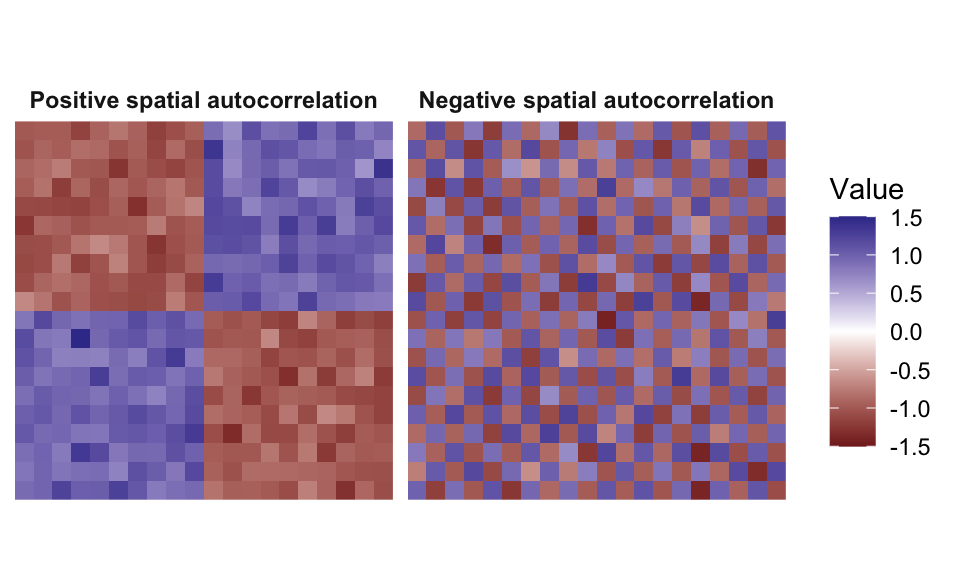
In the left panel, locations with similar values form contiguous groups. High values are generally connected to high values, and low values are generally connected to low values. This pattern illustrates positive spatial autocorrelation.

Positive spatial autocorrelation may arise because neighboring areas share economic, social, environmental, or institutional characteristics. It may also be generated by interaction across boundaries. Observing the pattern alone does not distinguish between these explanations.

In the right panel, high and low values alternate across the grid. Each unit tends to be connected to units displaying values of the opposite sign. This pattern illustrates negative spatial autocorrelation.

Negative spatial autocorrelation may arise in settings involving spatial competition, mutually exclusive land uses, alternating allocation rules, or other mechanisms that generate contrast between connected locations. As with positive autocorrelation, the observed pattern does not by itself identify the underlying mechanism.

ImportantSpatial autocorrelation is evidence of association, not causality

A measure of spatial autocorrelation summarizes how observed values align with a chosen spatial structure. It does not establish that a change in one unit causes a change in another. Similar spatial patterns can be generated by direct interaction, shared determinants, omitted variables, common shocks, sorting, or institutional boundaries. Causal or structural interpretation requires assumptions beyond the autocorrelation statistic itself.

The two panels are deliberately simplified. Real spatial data rarely display such perfectly organized patterns, and visual inspection alone cannot determine whether the observed arrangement is unusual under a specified null model. Formal measurement requires both a spatial weights matrix and a statistic such as Moran’s \(I\), which are developed later in the chapter.

1.2 The Spatial Weights Matrix

A central issue in spatial econometrics is how to represent the connections among spatial units without assigning an unrestricted interaction coefficient to every ordered pair of observations. As discussed in Section 1.1.1, an unrestricted system such as Equation 1.3 quickly introduces more parameters than can be identified from a single cross section. A parsimonious representation must therefore answer two related questions:

1. Which spatial units are considered connected?
2. How strong is each connection relative to the others?

The standard device is the spatial weights matrix, denoted by \(\mathbf W\). Suppose that the system contains \(n\) spatial units. Then \(\mathbf W\) is an \(n\times n\) matrix, \[ \mathbf W= \begin{pmatrix} w_{11} & w_{12} & \cdots & w_{1n}\\ w_{21} & w_{22} & \cdots & w_{2n}\\ \vdots & \vdots & \ddots & \vdots\\ w_{n1} & w_{n2} & \cdots & w_{nn} \end{pmatrix}, \tag{1.5}\] where the generic element \(w_{ij}\) measures the strength of the connection from unit \(j\) to unit \(i\). Reading the matrix by rows, row \(i\) shows which units \(j\) are connected to unit \(i\) and the weight assigned to each connection. Reading it by columns, column \(j\) shows the units \(i\) for which unit \(j\) appears as a connected unit and the weight assigned to that connection in each case.

Definition 1.1 (Spatial Weights Matrix) Let \(n\) denote the number of spatial units. A spatial weights matrix is an \(n\times n\) matrix \[ \mathbf W=(w_{ij}), \] whose elements are assigned according to a prespecified rule describing the connections among the units. In the standard case considered in this chapter, \[ w_{ij}\geq 0 \qquad\text{and}\qquad w_{ii}=0, \qquad i,j=1,\ldots,n. \]

The zero diagonal excludes a unit from its own set of immediate neighbors. That is, a spatial unit is not considered its own neighbor. Nonnegative elements indicate whether connections exist and how strong they are relative to one another. A value \(w_{ij}=0\) means that unit \(j\) is not regarded as directly connected to unit \(i\) under the selected rule, whereas \(w_{ij}>0\) represents a connection.

Nonnegative weights do not imply positive spatial autocorrelation. The matrix determines which relationships are considered relevant, but the observed data or the parameters of a spatial model determine whether connected units tend to have similar or dissimilar outcomes. Two locations may receive a positive weight because they share a border and nevertheless display negative spatial autocorrelation.

The matrix may be:

• binary, when it records only whether a connection exists;
• weighted, when its positive elements also measure relative connection strength;
• symmetric, when \(w_{ij}=w_{ji}\);
• asymmetric, when the direction of the connection matters.

Although geographic proximity is common, \(\mathbf W\) need not represent physical distance alone. Its elements may be based on common borders, travel times, migration, commuting, trade, input–output relationships, transport links, social networks, or other connections justified by the problem under study. The matrix is therefore part of the substantive specification of the model rather than a purely computational object.

ImportantKnown, fixed, and exogenous are different assumptions

Throughout most of this book, the spatial weights matrix \(\mathbf W\) is assumed to be observed and the econometric analysis is conducted conditionally on its realized values. These conventions simplify the analysis, but they should not be confused with an assumption of economic exogeneity.

The three concepts refer to different questions:

• Known asks whether the researcher observes the elements of \(\mathbf W\). For example, a contiguity matrix constructed from an observed map is known once the boundaries of the spatial units have been specified.

• Fixed or conditioned upon asks how \(\mathbf W\) is treated in the statistical analysis. Conditional inference regards the realized matrix as given and studies the randomness coming from the outcome and the explanatory variables, rather than from repeated realizations of the spatial network.

• Exogenous asks how the connections represented by \(\mathbf W\) were formed. Exogeneity requires that network formation not depend on unobserved determinants of the outcome in a way that creates correlation between \(\mathbf W\) and the model’s disturbances.

The distinction is important because observing a network does not explain why that network arose. For instance, a matrix based on commuting flows may be fully observed and treated as fixed. Nevertheless, those flows may partly reflect unobserved employment opportunities, productivity, or local amenities that also affect the outcome under study. In that case, conditioning on the observed matrix does not by itself remove the resulting endogeneity.

Thus, a spatial weights matrix may be known and treated as fixed while still being endogenous from an economic perspective. Unless stated otherwise, this book treats \(\mathbf W\) as known and fixed and assumes that it is sufficiently exogenous for the econometric model being considered. Models with endogenous network formation require additional assumptions and methods and are beyond the scope of this chapter.

The remainder of this section introduces two broad construction principles:

1. contiguity-based weights, which use shared polygon boundaries or vertices;
2. distance-based weights, which use geographic separation or a related measure of proximity.

This classification is convenient rather than exhaustive. The appropriate construction should be chosen to represent the mechanism that links the spatial units.

1.2.1 Weights Based on Boundaries

When spatial units are represented as areas on a map, such as municipalities, counties, or countries, two units can be defined as neighbors when their boundaries touch. Depending on the contiguity criterion, they may need to share a boundary segment or only a common point. This rule produces a binary contiguity matrix: \[ w_{ij}= \begin{cases} 1, & \text{if unit $j$ is contiguous to unit $i$},\\ 0, & \text{otherwise}. \end{cases} \tag{1.6}\]

Contiguity is usually reciprocal: if unit \(i\) is a neighbor of unit \(j\), then unit \(j\) is also a neighbor of unit \(i\). The resulting binary matrix is therefore symmetric. Three criteria can be used to determine what kind of contact is sufficient for two areas to be considered neighbors: rook, bishop, and queen contiguity. Rook and queen contiguity are the conventions most commonly used in empirical applications, whereas bishop contiguity is mainly useful for comparison and illustration.

1.2.1.1 Rook Contiguity

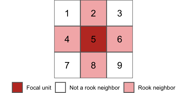
Under rook contiguity, two spatial units are neighbors when they share a common border. The name comes from the rook in chess: a rook moves only horizontally or vertically, not diagonally. In the same way, if we focus on the central unit of a regular \(3\times3\) grid, its rook neighbors are the four units located directly above, below, to the left, and to the right. For example, in Figure 1.3, the focal unit is Region 5. Using the rook rule, its rook neighbors are Regions 2, 4, 6, and 8.

Figure 1.3: Rook contiguity in a regular grid

For this grid, the corresponding \(9\times9\) binary matrix is \[ \mathbf W_R= \begin{pmatrix} 0 & 1 & 0 & 1 & 0 & 0 & 0 & 0 & 0\\ 1 & 0 & 1 & 0 & 1 & 0 & 0 & 0 & 0\\ 0 & 1 & 0 & 0 & 0 & 1 & 0 & 0 & 0\\ 1 & 0 & 0 & 0 & 1 & 0 & 1 & 0 & 0\\ 0 & 1 & 0 & 1 & 0 & 1 & 0 & 1 & 0\\ 0 & 0 & 1 & 0 & 1 & 0 & 0 & 0 & 1\\ 0 & 0 & 0 & 1 & 0 & 0 & 0 & 1 & 0\\ 0 & 0 & 0 & 0 & 1 & 0 & 1 & 0 & 1\\ 0 & 0 & 0 & 0 & 0 & 1 & 0 & 1 & 0 \end{pmatrix}. \tag{1.7}\]

In this matrix, the fifth row has ones in columns 2, 4, 6, and 8, showing that Region 5 is connected to those four regions. The fifth column displays the same pattern because rook contiguity is reciprocal: if Region 2 is a rook neighbor of Region 5, then Region 5 is also a rook neighbor of Region 2, and similarly for Regions 4, 6, and 8.

NoteA practical note on polygon boundaries

On an ideal map, deciding whether two areas share a border is straightforward. In real spatial data, however, polygon boundaries are stored as sets of coordinates. Two boundaries that appear to touch on a map may contain a very small gap, overlap slightly, or be represented by points that do not match exactly. These imperfections can affect the neighbors identified by the software. For example, two municipalities that should share a border may not be recognized as rook neighbors, while small geometric errors may occasionally create an unexpected connection. For this reason, the neighborhood structure should always be inspected after it has been constructed. A map of the connections, together with a review of units with unusually few or many neighbors, can help detect problems before the weights matrix is used in the analysis. Some computational routines identify rook contiguity by checking whether polygons share more than one boundary point. In digital maps, this criterion does not always coincide perfectly with the ideal notion of sharing a continuous border segment.

1.2.1.2 Bishop Contiguity

Under bishop contiguity, imagine the movement of a bishop on a chessboard. A bishop moves diagonally, so it reaches squares that touch the current square only at a corner. In the same way, two spatial units are bishop neighbors when they meet at a common point but do not share a border.

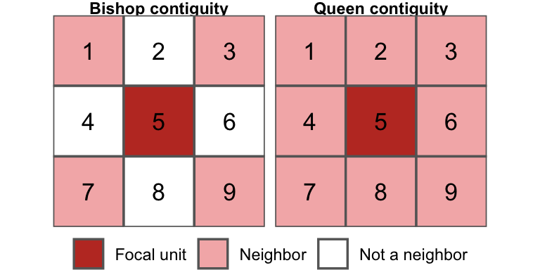
For the central unit in the \(3\times3\) grid, the bishop neighbors are Regions 1, 3, 7, and 9, as shown in the left panel of Figure 1.4. The corresponding binary matrix is \[ \mathbf W_B= \begin{pmatrix} 0 & 0 & 0 & 0 & 1 & 0 & 0 & 0 & 0\\ 0 & 0 & 0 & 1 & 0 & 1 & 0 & 0 & 0\\ 0 & 0 & 0 & 0 & 1 & 0 & 0 & 0 & 0\\ 0 & 1 & 0 & 0 & 0 & 0 & 0 & 1 & 0\\ 1 & 0 & 1 & 0 & 0 & 0 & 1 & 0 & 1\\ 0 & 1 & 0 & 0 & 0 & 0 & 0 & 1 & 0\\ 0 & 0 & 0 & 0 & 1 & 0 & 0 & 0 & 0\\ 0 & 0 & 0 & 1 & 0 & 1 & 0 & 0 & 0\\ 0 & 0 & 0 & 0 & 1 & 0 & 0 & 0 & 0 \end{pmatrix}. \tag{1.8}\]

The fifth row has ones in columns 1, 3, 7, and 9, showing that Region 5 is connected diagonally to those four regions. The same connections also appear in the fifth column. This is because bishop contiguity is reciprocal: if Region 1 is a bishop neighbor of Region 5, then Region 5 is also a bishop neighbor of Region 1. Therefore, \(w_{ij}=w_{ji}\), and the binary bishop-contiguity matrix is symmetric: \(\mathbf W_B=\mathbf W_B^\top\).

Bishop contiguity is less common in empirical applications because touching only at a corner often provides a weaker reason for two areas to interact than sharing a border. Corner contacts may also be sensitive to small differences in how polygon boundaries are drawn. Nevertheless, bishop contiguity is useful for distinguishing diagonal connections from side-sharing connections and may be appropriate when meeting at a particular junction has substantive importance.

1.2.1.3 Queen Contiguity

Under queen contiguity, imagine the movement of a queen on a chessboard. Unlike the rook or the bishop, the queen can move horizontally, vertically, and diagonally. In the same way, two spatial units are queen neighbors when they share either a border or a corner.

For the central unit in the regular \(3\times3\) grid, queen contiguity combines the four rook neighbors—Regions 2, 4, 6, and 8—with the four bishop neighbors—Regions 1, 3, 7, and 9. Region 5 is therefore connected to all eight surrounding regions, as shown in the right panel of Figure 1.4.

Figure 1.4: Bishop and queen contiguity in a regular grid

The corresponding binary queen-contiguity matrix is \[ \mathbf W_Q= \begin{pmatrix} 0 & 1 & 0 & 1 & 1 & 0 & 0 & 0 & 0\\ 1 & 0 & 1 & 1 & 1 & 1 & 0 & 0 & 0\\ 0 & 1 & 0 & 0 & 1 & 1 & 0 & 0 & 0\\ 1 & 1 & 0 & 0 & 1 & 0 & 1 & 1 & 0\\ 1 & 1 & 1 & 1 & 0 & 1 & 1 & 1 & 1\\ 0 & 1 & 1 & 0 & 1 & 0 & 0 & 1 & 1\\ 0 & 0 & 0 & 1 & 1 & 0 & 0 & 1 & 0\\ 0 & 0 & 0 & 1 & 1 & 1 & 1 & 0 & 1\\ 0 & 0 & 0 & 0 & 1 & 1 & 0 & 1 & 0 \end{pmatrix}. \tag{1.9}\]

The fifth row has ones in every column except column 5. This shows that Region 5 is a queen neighbor of all eight surrounding regions, but not of itself.

In this regular grid, every queen connection is either a rook connection or a bishop connection. The two types do not overlap: two distinct cells either share a side or meet only at a corner. Therefore, \[ \mathbf W_Q = \mathbf W_R+\mathbf W_B. \tag{1.10}\]

For example, the fifth row of \(\mathbf W_R\) identifies Regions 2, 4, 6, and 8, while the fifth row of \(\mathbf W_B\) identifies Regions 1, 3, 7, and 9. Adding the two rows gives the fifth row of \(\mathbf W_Q\), which identifies all eight queen neighbors of Region 5.

Similar to rook and bishop, queen contiguity is reciprocal. If Region \(i\) shares a border or a corner with Region \(j\), then Region \(j\) shares the same border or corner with Region \(i\). Hence, \(w_{ij}=w_{ji}\), and the binary queen-contiguity matrix is symmetric.

For irregular polygons, the same basic idea applies: two areas are queen neighbors whenever they share a border or meet at at least one point. Because queen contiguity also includes corner contacts, it generally gives each unit more neighbors than rook contiguity.

The choice between rook and queen contiguity should reflect how interaction is expected to occur. If sharing a border is necessary for meaningful contact, rook contiguity may be more appropriate. If meeting at a corner is also enough to create a relevant connection, queen contiguity may provide a better description. The choice should be guided by the application rather than by which matrix produces more convenient empirical results.

1.2.2 Weights Based on Distance

Many spatial datasets locate observations as points on a map. Cities, stores, schools, and monitoring stations may already be represented by points. When the observations are areas, such as municipalities, counties, or countries, a representative point can be chosen for each area.

A location on a map is described by a pair of coordinates. On a geographic map, these coordinates are usually longitude and latitude. On a projected map, they are typically horizontal and vertical coordinates measured in units such as meters or kilometers.

Once the locations of two units are known, we can measure how far apart they are. The appropriate measure depends on the question being studied. Geographic distance, travel time, transportation cost, and economic distance may produce very different notions of which units are close to one another.

1.2.2.1 Distance on a Flat Map

Suppose that units \(i\) and \(j\) are located at coordinates \((x_i,y_i)\) and \((x_j,y_j)\) on a projected map. The most familiar measure is the Euclidean distance, \[ d_{ij}^{\mathrm E} = \sqrt{(x_i-x_j)^2+(y_i-y_j)^2}. \tag{1.11}\]

This is the straight-line distance between the two locations. It is the length of the direct line that joins the two points on a flat map.

A different measure is the Manhattan distance, \[ d_{ij}^{\mathrm M} = |x_i-x_j|+|y_i-y_j|. \tag{1.12}\]

Instead of measuring a direct line, Manhattan distance adds the horizontal and vertical movements needed to travel between the two points. The name comes from the regular street grid associated with Manhattan, where a traveler may need to move along streets rather than directly across city blocks.

Figure 1.5 compares the two measures. Under Euclidean distance, locations that are equally far from the center form a circle. Under Manhattan distance, they form a diamond because distance is accumulated through horizontal and vertical movement.

Figure 1.5: Equal-distance contours under Euclidean and Manhattan distance

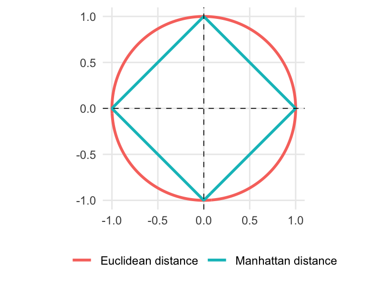
Euclidean and Manhattan distances treat the map as a flat surface. They are appropriate when the coordinates come from a suitable projected coordinate system and are measured in meaningful distance units, such as meters or kilometers.

They should not normally be applied directly to longitude and latitude measured in degrees. One degree of longitude does not represent the same surface distance everywhere on Earth: the distance between lines of longitude becomes smaller as one moves toward the poles.

1.2.2.2 Distance on the Earth’s Surface

When two locations are far apart, the curvature of the Earth becomes important. A distance calculated as though the map were flat may then give a misleading picture of their geographic separation.

The great-circle distance measures the shortest path between two locations along the surface of a sphere. It is therefore more appropriate for long-distance geographic connections, such as those between countries, ports, or airports.

Let \(\lambda_i\) and \(\lambda_j\) denote longitude, and let \(\phi_i\) and \(\phi_j\) denote latitude, all expressed in radians. Treating the Earth as a sphere, the great-circle distance is \[ d_{ij}^{\mathrm{GC}} = r_E \arccos\left[ \sin(\phi_i)\sin(\phi_j) + \cos(\phi_i)\cos(\phi_j) \cos(\lambda_i-\lambda_j) \right], \tag{1.13}\] where \(r_E\) is the Earth’s radius.

The main idea is that this measure follows the curvature of the Earth instead of treating the map as a flat plane. It can therefore provide a better measure of geographic separation for air or sea connections over long distances. It does not necessarily equal the route actually traveled, however. Flight paths, shipping routes, weather conditions, and transportation networks may lead to a longer journey.

In empirical work, distances should normally be calculated with spatial software that recognizes the coordinate reference system of the data. This is safer than applying a formula manually without first checking how the locations are represented.

After distances have been calculated, they must be converted into connections or weights. The following constructions are common.

1.2.2.3 Inverse-Distance Weights

Inverse-distance weights are based on the idea that nearby units are more strongly connected than distant units. The raw weight assigned to the pair \(i,j\) is \[ w_{ij}^{*} = \begin{cases} d_{ij}^{-\alpha}, & i\neq j,\\ 0, & i=j, \end{cases} \qquad \alpha>0. \tag{1.14}\]

The parameter \(\alpha\) determines how strongly distance reduces the connection. Its role can be seen by comparing two units, \(j\) and \(k\), located at different distances from unit \(i\): \[ \frac{w_{ij}^{*}}{w_{ik}^{*}} = \left( \frac{d_{ik}}{d_{ij}} \right)^\alpha. \]

Suppose, for example, that unit \(k\) is twice as far from unit \(i\) as unit \(j\). Then:

• if \(\alpha=1\), unit \(k\) receives one-half of the weight assigned to unit \(j\);
• if \(\alpha=2\), it receives only one-quarter;
• if \(\alpha=0.5\), it receives approximately \(1/\sqrt{2}\) of that weight.

A larger value of \(\alpha\) is appropriate when interaction is expected to be highly local and to weaken quickly with distance. In this case, nearby units receive much more weight than moderately distant ones. This may be reasonable, for example, when transportation costs, commuting constraints, or other spatial frictions rise sharply with distance.

A smaller value of \(\alpha\) is appropriate when distance is expected to reduce interaction more gradually. More distant units then retain a meaningful weight, which may be reasonable when the relevant connections extend over a broader geographic area.

The choice of \(\alpha\) should therefore reflect the mechanism being studied. It should not be selected simply because a particular value produces stronger statistical results. When theory does not provide a clear value, the researcher can report whether the main conclusions are robust to several plausible rates of distance decay.

Setting \(w_{ii}^{*}=0\) is necessary because \(d_{ii}=0\) and the inverse of zero is undefined. Very small distances between distinct observations can also produce extremely large raw weights, so duplicated or nearly duplicated coordinates should be checked.

1.2.2.4 Negative-Exponential Weights

An alternative way to represent distance decay is the negative-exponential function: \[ w_{ij}^{*} = \begin{cases} \exp(-\alpha d_{ij}), & i\neq j,\\ 0, & i=j, \end{cases} \qquad \alpha>0. \tag{1.15}\]

The term negative exponential refers to the negative sign in the exponent. It does not mean that the weights themselves are negative. Because \(0<\exp(-\alpha d_{ij})\leq1\) for every finite positive distance, all off-diagonal weights remain positive.

As with inverse-distance weights, nearby units receive more weight than distant units. The difference lies in how quickly the connection declines. To see this, consider increasing the distance from \(d\) to \(d+\Delta\). Under the exponential specification, \[ \frac{\exp[-\alpha(d+\Delta)]} {\exp(-\alpha d)} = \exp(-\alpha\Delta). \]

Thus, adding the same amount of distance always reduces the weight by the same proportion. For example, if an additional 10 kilometers reduces a connection by 20 percent, another 10 kilometers produces the same proportional reduction, regardless of the initial distance.

This differs from inverse-distance weights. Under \(w_{ij}^{*}=d_{ij}^{-\alpha}\), multiplying a distance by a factor \(c\) changes its weight according to \[ \frac{(cd_{ij})^{-\alpha}} {d_{ij}^{-\alpha}} = c^{-\alpha}. \]

Therefore, inverse-distance weights are naturally interpreted in terms of relative distance. If one unit is twice as far away as another, the ratio between their weights depends only on \(\alpha\), regardless of whether the distances are 10 and 20 kilometers or 100 and 200 kilometers.

The two functions also differ in their behavior over long distances. Inverse-distance weights decline gradually, so distant units may continue to receive non-negligible weight. Exponential weights decline much more rapidly, concentrating the connection on nearby units. For this reason:

• inverse-distance weights may be appropriate when interactions extend over a broad geographic area and decay gradually;
• exponential weights may be preferable when interactions are expected to be strongly local and to become negligible beyond a relatively short distance.

For example, broad information flows or interregional economic relationships may exhibit gradual decay. By contrast, local commuting, access to nearby services, or environmental effects with a limited geographic reach may be better represented by a faster exponential decline. These are only guiding examples; the appropriate function depends on the mechanism studied.

The parameter \(\alpha\) controls the speed of exponential decay. A larger \(\alpha\) assigns relatively more weight to the nearest units and causes distant connections to disappear more quickly. A smaller \(\alpha\) allows meaningful weights to persist over a wider area.

An equivalent and often more intuitive parameterization is \[ w_{ij}^{*} = \exp\left(-\frac{d_{ij}}{h}\right), \qquad h>0, \] where \[ h=\frac{1}{\alpha}. \]

The parameter \(h\) has the same units as distance and describes the geographic scale over which connections decline. When \(d_{ij}=h\), \[ w_{ij}^{*} = \exp(-1) \approx0.368. \]

A larger \(h\) therefore represents connections that extend over longer distances, whereas a smaller \(h\) represents highly localized connections.

NoteDistance units matter

In the exponential specification, the decay parameter depends on the units in which distance is measured. A value of \(\alpha\) used with kilometers cannot be used unchanged when the same distances are expressed in meters. Under the parameterization \(\exp(-d_{ij}/h)\), both \(d_{ij}\) and \(h\) must be measured in the same units. This issue is less consequential for row-standardized inverse-distance weights: multiplying every distance by the same constant multiplies all raw weights by a common factor, which disappears after row standardization. For exponential weights, changing the distance units changes the relative weights unless \(\alpha\) or \(h\) is adjusted accordingly.

Unlike inverse-distance weights, exponential weights remain bounded when two distinct observations are extremely close: as \(d_{ij}\) approaches zero, \[ \exp(-\alpha d_{ij}) \longrightarrow1. \]

Duplicated or nearly duplicated coordinates should nevertheless be checked, because such observations may receive substantially more weight than all other units.

Both inverse-distance and exponential specifications connect every pair of units whenever all distances are finite. They therefore produce dense matrices unless they are combined with a distance cutoff or another neighborhood rule. Row standardization (see Section 1.3) does not eliminate the difference between the two decay functions: it makes each row sum to one, but the distribution of that total weight across nearby and distant units remains different.

Neither specification is universally preferable. The distance metric, decay function, and decay parameter should reflect the interaction mechanism being represented by the spatial weights matrix (Anselin and Rey 2014). When no single choice is clearly implied by theory, conclusions should be examined across a small set of economically plausible specifications.

1.2.2.5 \(k\)-Nearest-Neighbor Weights

A \(k\)-nearest-neighbor rule connects each spatial unit to the \(k\) units located closest to it. Imagine drawing a circle around unit \(i\) and gradually expanding it until exactly \(k\) other units have been reached. Those units form the set \(\mathcal N_k(i)\).

The corresponding binary weights are \[ w_{ij}^{*} = \begin{cases} 1, & j\in\mathcal N_k(i),\\ 0, & \text{otherwise}. \end{cases} \tag{1.16}\]

Thus, each row of \(\mathbf W^{*}\) contains exactly \(k\) ones, provided that distances are available and ties are resolved. This guarantees that every unit has neighbors and therefore avoids spatial isolates.

The value of \(k\) determines how local the resulting neighborhood structure is. A small value of \(k\) restricts each unit to only its closest surroundings. This may be appropriate when interaction is expected to be highly local, but it can also produce a weakly connected or fragmented spatial structure. A larger value of \(k\) creates broader neighborhoods and usually strengthens connectivity, but it may also link units that are too far apart to be substantively related.

The appropriate value of \(k\) therefore depends on the mechanism being studied. For example, a small \(k\) may be reasonable when only the nearest competing store, hospital, or municipality is expected to matter. A larger \(k\) may be more appropriate when interaction takes place across a wider regional system.

A useful feature of this construction is that every unit has the same number of neighbors. The geographic reach of those neighborhoods, however, need not be the same. In a densely populated area, the \(k\) nearest neighbors may all be located nearby. In a sparsely populated area, reaching the same number of neighbors may require covering a much larger distance.

The \(k\)-nearest-neighbor relation is not generally reciprocal. Unit \(j\) may be one of the \(k\) closest units to unit \(i\), while unit \(i\) is not one of the \(k\) closest units to unit \(j\). Therefore, \[ w_{ij}^{*}>0 \quad\not\Rightarrow\quad w_{ji}^{*}>0. \]

For example, suppose that the closest unit to \(A\) is \(B\), but the closest unit to \(B\) is \(C\). With \(k=1\), \(B\) is selected as a neighbor of \(A\), but \(A\) is not selected as a neighbor of \(B\). The resulting binary matrix is asymmetric.

The relation can be made symmetric, but doing so changes the original neighbor rule. One possibility is to treat \(i\) and \(j\) as neighbors whenever either unit selects the other. Another is to require that both units select each other. These alternatives generally produce different numbers of neighbors and should be regarded as separate modeling choices.

Ties may also occur when several units are located at exactly the same distance as the \(k\)th neighbor. The researcher must then specify whether all tied units are included or whether a fixed rule is used to retain exactly \(k\) neighbors.

1.2.2.6 Distance-Band Weights

A distance-band rule connects each unit to all other units located within a specified distance. The idea is similar to drawing a circle of radius \(d_{\max}\) around each location: every unit falling inside that circle is treated as a neighbor.

The corresponding binary weights are \[ w_{ij}^{*} = \begin{cases} 1, & 0<d_{ij}\leq d_{\max},\\ 0, & \text{otherwise}. \end{cases} \tag{1.17}\]

The threshold \(d_{\max}\) determines the geographic reach of the neighborhood. A small threshold produces highly local neighborhoods, but some units may have no neighbors. A large threshold connects more units and reduces the risk of isolates, but it may also include connections that are too distant to represent the mechanism under study.

Unlike the \(k\)-nearest-neighbor rule, a distance band does not force every unit to have the same number of neighbors. Units in dense areas may have many neighbors within the threshold, whereas units in sparse areas may have only a few. This difference can be substantively meaningful when the same geographic range is expected to apply everywhere.

When distance is symmetric, \(d_{ij}=d_{ji}\), the neighbor relation is reciprocal. If unit \(j\) lies within distance \(d_{\max}\) of unit \(i\), then unit \(i\) lies within the same distance of unit \(j\). Consequently, \(w_{ij}^{*}=w_{ji}^{*}\), and the binary distance-band matrix is symmetric.

To ensure that every unit has at least one neighbor, the distance threshold must be at least as large as the greatest nearest-neighbor distance in the sample: \[ d_{\max} \geq \max_i \left\{ \min_{j\neq i}d_{ij} \right\}. \tag{1.18}\]

The expression can be understood in two steps. First, for each unit \(i\), find the distance to its closest neighbor: \(\min_{j\neq i}d_{ij}\). Then identify the largest of these nearest-neighbor distances across all units. Choosing \(d_{\max}\) at least this large guarantees that even the most isolated unit reaches its closest neighbor.

This condition prevents rows with no neighbors, but it does not guarantee that all units belong to a single connected spatial system. The data may still contain two or more groups that are internally connected but remain separated from one another. The resulting neighborhood structure should therefore be inspected for both isolates and disconnected groups.

NoteChoosing a neighborhood rule

A spatial weights matrix begins with a substantive question: which other units should be considered relevant for unit \(i\)?

Different constructions answer this question in different ways:

• contiguity weights connect areas whose boundaries touch;
• distance-decay weights allow connections to weaken gradually with distance;
• \(k\)-nearest-neighbor weights give every unit the same number of neighbors;
• distance-band weights give every unit the same geographic range;
• flow- or network-based weights use observed economic or social connections.

These rules are not interchangeable. For example, \(k\)-nearest neighbors may connect a rural municipality to units located far away in order to reach the required number of neighbors. A distance band avoids this variation in geographic reach, but it may give urban units many neighbors and rural units very few.

There is therefore no spatial weights matrix that is universally correct. The choice should follow the mechanism being studied. Robustness analysis is valuable, but the alternatives being compared should all remain economically and geographically plausible.

1.3 Row-Standardized Spatial Weights Matrix

The weights constructed in the previous sections need not have the same total magnitude in every row. This occurs naturally because spatial units may have different numbers of neighbors or different total intensities of connection.

Consider, for example, a binary contiguity matrix. If unit \(i\) has three neighbors, the elements in row \(i\) sum to three. If unit \(r\) has six neighbors, the elements in row \(r\) sum to six. The two rows are therefore measured on different scales, even though both were constructed using the same contiguity rule.

Row standardization, also called row normalization, places every nonzero row on a common scale by making its elements sum to one. For binary weights, this means that a unit with three neighbors assigns weight \(1/3\) to each of them, whereas a unit with six neighbors assigns weight \(1/6\) to each.

This transformation is useful for two related reasons. First, it makes the weights comparable across units with different numbers or intensities of connections. Second, it controls the total weight assigned by each row. This mathematical property will become important in later chapters when we study powers of the spatial weights matrix, spatial multipliers, parameter spaces, and asymptotic sequences of spatial models.

Row standardization does not, by itself, guarantee all the regularity conditions required for asymptotic analysis. It does, however, impose the useful restriction that the absolute row sums remain uniformly controlled.

To distinguish the original weights from their standardized version, let \[ \mathbf W^{*} = \left(w_{ij}^{*}\right) \] denote the original \(n\times n\) spatial weights matrix. The elements of \(\mathbf W^{*}\) may be binary or may measure distance, trade, commuting, migration, or another form of connectivity.

For each unit \(i\), define the sum of the original weights in row \(i\) as \[ s_i = \sum_{j=1}^{n}w_{ij}^{*}. \tag{1.19}\]

When \(s_i>0\), the standardized weight is \[ w_{ij} = \frac{w_{ij}^{*}}{s_i} = \frac{w_{ij}^{*}} {\displaystyle\sum_{k=1}^{n}w_{ik}^{*}}. \tag{1.20}\]

The denominator is the total original weight in row \(i\). Dividing each element by this total changes the scale of the row but preserves the relative importance of its connections. In particular, for any two units \(j\) and \(k\) such that \(w_{ik}^{*}>0\), \[ \frac{w_{ij}}{w_{ik}} = \frac{w_{ij}^{*}}{w_{ik}^{*}}. \tag{1.21}\]

Thus, if unit \(j\) originally receives twice as much weight as unit \(k\) in row \(i\), it continues to receive twice as much weight after standardization.

Let \[ \mathbf D = \operatorname{diag}(s_1,\ldots,s_n). \]

If every row has a strictly positive sum, the complete transformation can be written as \[ \mathbf W = \mathbf D^{-1}\mathbf W^{*}. \tag{1.22}\]

From this point onward, unless stated otherwise, \(\mathbf W\) denotes the spatial weights matrix after the selected coding or normalization has been applied.

A unit for which \(s_i=0\) has no neighbors under the selected rule and is usually called a spatial isolate or island. Row standardization is not defined for such a row because it would require division by zero. The researcher must then reconsider the neighbor rule, remove the unit when this is substantively defensible, or retain a zero row under an explicitly stated convention. The consequences of retaining a zero row will be discussed when spatially weighted variables are introduced in the next section.

For every non-isolated unit, the standardized weights sum to one: \[ \sum_{j=1}^{n}w_{ij}=1. \tag{1.23}\]

Indeed, \[ \begin{aligned} \sum_{j=1}^{n}w_{ij} = \sum_{j=1}^{n}\frac{w_{ij}^{*}}{s_i} = \frac{1}{s_i} \sum_{j=1}^{n}w_{ij}^{*} = \frac{s_i}{s_i} &=1. \end{aligned} \]

If the original weights are nonnegative, then \(0\leq w_{ij}\leq1\). Moreover, if all \(n\) rows have positive sums, the sum of all elements of the standardized matrix is \[ \begin{aligned} S_0 = \sum_{i=1}^{n}\sum_{j=1}^{n}w_{ij} = \sum_{i=1}^{n}1 =n. \end{aligned} \tag{1.24}\]

Row standardization places all rows on a common scale, but this transformation is not substantively neutral. Suppose that the original weights measure trade flows. A region with total trade equal to 100 and another with total trade equal to 1,000 both have standardized row sums equal to one. The transformation preserves how each region distributes its trade across partners, but it removes the difference in their total trade intensity.

More generally, row standardization preserves the composition of each row while discarding its original total magnitude. Whether this is desirable depends on the meaning of the original weights and on the economic mechanism being represented.

The resulting matrix belongs to an important class of matrices.

Definition 1.2 (Row-Stochastic Matrix) A real \(n\times n\) matrix \(\mathbf A=(a_{ij})\) is called a row-stochastic matrix, or Markov matrix, if:

1. \(a_{ij}\geq0\) for every \(i,j=1,\ldots,n\); and
2. \(\sum_{j=1}^{n}a_{ij}=1\) for every \(i=1,\ldots,n\).

Every row-standardized spatial weights matrix without zero rows is therefore row-stochastic. This classification is not merely terminological. The common row sum imposes useful restrictions on the eigenvalues of the matrix, which will later help us study repeated spatial connections and the invertibility of spatial multipliers.

The first spectral consequence follows directly from the fact that every row sums to one. A second consequence is that no eigenvalue can have modulus greater than one.

Theorem 1.1 (Eigenvalues of a Row-Stochastic Matrix) Let \(\mathbf A\) be an \(n\times n\) row-stochastic matrix. Then:

1. \(\omega=1\) is an eigenvalue of \(\mathbf A\); and
2. every eigenvalue \(\omega\) of \(\mathbf A\) satisfies \(|\omega|\leq1\).

Proof. Let \(\boldsymbol\iota_n\) denote the \(n\times1\) vector of ones. Because every row of \(\mathbf A\) sums to one, \[ \mathbf A\boldsymbol\iota_n = \boldsymbol\iota_n. \]

Therefore, \(\boldsymbol\iota_n\) is a right eigenvector associated with the eigenvalue \(\omega=1\).

Now let \(\omega\) be any eigenvalue of \(\mathbf A\), and let \(\mathbf v\neq\mathbf0\) be an associated eigenvector. Thus, \[ \mathbf A\mathbf v = \omega\mathbf v. \]

Choose an index \(k\) such that \[ |v_k| = \max_{1\leq i\leq n}|v_i|. \]

Because \(\mathbf v\neq\mathbf0\), we have \(|v_k|>0\). The \(k\)th element of the eigenvalue equation is \[ \sum_{j=1}^{n}a_{kj}v_j = \omega v_k. \]

Taking absolute values and applying the triangle inequality gives \[ \begin{aligned} |\omega|\,|v_k| &= \left|\sum_{j=1}^{n}a_{kj}v_j\right| \\ &\leq \sum_{j=1}^{n}a_{kj}|v_j|. \end{aligned} \]

By the definition of \(k\), \[ |v_j|\leq|v_k| \qquad \text{for every }j=1,\ldots,n. \]

Since \(a_{kj}\geq0\), \[ \begin{aligned} \sum_{j=1}^{n}a_{kj}|v_j| &\leq \sum_{j=1}^{n}a_{kj}|v_k| \\ &= |v_k|\sum_{j=1}^{n}a_{kj} \\ &= |v_k|. \end{aligned} \]

Combining the inequalities yields \[ |\omega|\,|v_k| \leq |v_k|. \]

Division by \(|v_k|>0\) gives \[ |\omega|\leq1. \]

The theorem has the following immediate consequence.

Corollary 1.1 (Spectral Radius of a Row-Stochastic Matrix) If \(\mathbf A\) is row-stochastic, then \[ \varrho(\mathbf A)=1, \]

where \(\varrho(\mathbf A)\) denotes the spectral radius of \(\mathbf A\).

Proof. The spectral radius is \[ \varrho(\mathbf A) = \max_{1\leq h\leq n}|\omega_h|, \] where \(\omega_1,\ldots,\omega_n\) are the eigenvalues of \(\mathbf A\). The preceding theorem establishes that \(1\) is an eigenvalue, so \(\varrho(\mathbf A)\geq1\). It also establishes that every eigenvalue satisfies \(|\omega_h|\leq1\), so \(\varrho(\mathbf A)\leq1\). Therefore, \[ \varrho(\mathbf A)=1. \]

The eigenvalues of a row-stochastic matrix therefore lie in the closed unit disk of the complex plane. It is not generally correct to claim that they all belong to the real interval \([-1,1]\), because an asymmetric row-stochastic matrix may have complex eigenvalues.

There is, however, an important special case. Suppose that the original matrix \(\mathbf W^{*}\) is symmetric and has strictly positive row sums. Although \[ \mathbf W = \mathbf D^{-1}\mathbf W^{*} \] is generally asymmetric, it is similar to the symmetric matrix \[ \widetilde{\mathbf W} = \mathbf D^{-1/2} \mathbf W^{*} \mathbf D^{-1/2}. \tag{1.25}\]

Indeed, \[ \mathbf W = \mathbf D^{-1/2} \widetilde{\mathbf W} \mathbf D^{1/2}. \tag{1.26}\]

To verify the identity, substitute the definition of \(\widetilde{\mathbf W}\): \[ \begin{aligned} \mathbf D^{-1/2} \widetilde{\mathbf W} \mathbf D^{1/2} &= \mathbf D^{-1/2} \left( \mathbf D^{-1/2} \mathbf W^{*} \mathbf D^{-1/2} \right) \mathbf D^{1/2} \\ &= \mathbf D^{-1} \mathbf W^{*} \\ &= \mathbf W. \end{aligned} \]

Similar matrices have the same eigenvalues. Since \(\widetilde{\mathbf W}\) is real and symmetric, all its eigenvalues are real. Consequently, when the original matrix \(\mathbf W^{*}\) is symmetric, the eigenvalues of its row-standardized version \(\mathbf W\) are real and belong to \([-1,1]\).

Row standardization may also change the symmetry of the original matrix. Reciprocal neighborhood relations do not necessarily imply reciprocal standardized weights. For example, suppose that units \(i\) and \(j\) are connected and that the original binary weights satisfy \(w_{ij}^{*}=w_{ji}^{*}=1\). If unit \(i\) has two neighbors while unit \(j\) has five, then \[ w_{ij}=\frac{1}{2}, \qquad w_{ji}=\frac{1}{5}. \]

The connection remains reciprocal, but its standardized strength differs in the two directions because the two rows have different totals. Even if \(w_{ij}^{*}=w_{ji}^{*}\), the standardized weights satisfy \[ w_{ij} = \frac{w_{ij}^{*}}{s_i} \qquad\text{and}\qquad w_{ji} = \frac{w_{ji}^{*}}{s_j}. \]

Therefore, if \(s_i\neq s_j\), it is generally possible that \(w_{ij}\neq w_{ji}\).

1.4 Spatially Lagged Variables

Once a spatial weights matrix has been constructed, it can be used to summarize the values observed around each spatial unit. This summary is called a spatial lag.

The word lag should not be interpreted in its usual time-series sense. A temporal lag refers to the value of a variable in an earlier period. A spatial lag instead refers to values observed in other spatial units that are connected to the unit under consideration.

Let \[ \mathbf y = \begin{pmatrix} y_1\\ y_2\\ \vdots\\ y_n \end{pmatrix} \] be an \(n\times1\) vector containing one observation for each of the \(n\) spatial units.

Definition 1.3 (Spatial Lag) Given an \(n\times n\) spatial weights matrix \(\mathbf W\) and an \(n\times1\) vector \(\mathbf y\), the spatial lag of \(\mathbf y\) is \[ \mathbf y_{\mathrm L} = \mathbf W\mathbf y. \tag{1.27}\]

The \(i\)th element is \[ y_{\mathrm L,i} = \sum_{j=1}^{n}w_{ij}y_j. \tag{1.28}\]

The expression is easiest to understand by reading row \(i\) of \(\mathbf W\). Each positive element \(w_{ij}\) indicates that the value observed in unit \(j\) contributes to the spatial lag calculated for unit \(i\). The magnitude of \(w_{ij}\) determines how much weight that value receives.

Thus, \[ y_{\mathrm L,i} = w_{i1}y_1 + w_{i2}y_2 + \cdots + w_{in}y_n. \]

Because the diagonal elements of a spatial weights matrix are usually set equal to zero, \(w_{ii}=0\), the value \(y_i\) does not normally contribute to its own spatial lag. The spatial lag summarizes the values observed in the other units connected with unit \(i\).

The interpretation depends on how \(\mathbf W\) has been coded:

• with binary unstandardized weights, the spatial lag is the sum of the values observed in neighboring units;
• with row-standardized weights, the spatial lag is a weighted average of those values;
• with other nonbinary weights, it is a weighted sum whose interpretation depends on the meaning of the weights.

Consider a system with three spatial units. Let the original binary matrix be \[ \mathbf W^{*} = \begin{pmatrix} 0&1&0\\ 1&0&1\\ 0&1&0 \end{pmatrix}, \qquad \mathbf y = \begin{pmatrix} 10\\ 50\\ 30 \end{pmatrix}. \]

The first row of \(\mathbf W^{*}\) shows that Unit 1 is connected only to Unit 2. The second row shows that Unit 2 is connected to Units 1 and 3. The third row shows that Unit 3 is connected only to Unit 2.

Using the unstandardized matrix gives \[ \begin{aligned} \mathbf W^{*}\mathbf y &= \begin{pmatrix} 0&1&0\\ 1&0&1\\ 0&1&0 \end{pmatrix} \begin{pmatrix} 10\\ 50\\ 30 \end{pmatrix} \\ &= \begin{pmatrix} 50\\ 10+30\\ 50 \end{pmatrix} \\ &= \begin{pmatrix} 50\\ 40\\ 50 \end{pmatrix}. \end{aligned} \tag{1.29}\]

For Unit 1, the spatial lag is simply the value observed in Unit 2: \(y_{\mathrm L,1}=50\). For Unit 2, the spatial lag is the sum of the values observed in Units 1 and 3: \(y_{\mathrm L,2} = 10+30 = 40\). For Unit 3, the spatial lag is again the value observed in Unit 2: \(y_{\mathrm L,3}=50\).

Now row-standardize the matrix: \[ \mathbf W = \begin{pmatrix} 0&1&0\\ \frac12&0&\frac12\\ 0&1&0 \end{pmatrix}. \]

The corresponding spatial lag is \[ \begin{aligned} \mathbf W\mathbf y &= \begin{pmatrix} 0&1&0\\ \frac12&0&\frac12\\ 0&1&0 \end{pmatrix} \begin{pmatrix} 10\\ 50\\ 30 \end{pmatrix} \\ &= \begin{pmatrix} 50\\ \frac12(10)+\frac12(30)\\ 50 \end{pmatrix} \\ &= \begin{pmatrix} 50\\ 20\\ 50 \end{pmatrix}. \end{aligned} \tag{1.30}\]

The spatial lag for Unit 2 is now the average of the values observed in Units 1 and 3: \(y_{\mathrm L,2} = \frac12(10)+\frac12(30) = 20\). The difference between 40 and 20 is not a numerical accident. With binary unstandardized weights, the spatial lag adds the neighboring values. With row-standardized weights, it averages them.

For a non-isolated unit and nonnegative row-standardized weights, the spatial lag must lie between the smallest and largest values in its neighborhood: \[ \min_{j:w_{ij}>0}y_j \leq y_{\mathrm L,i} \leq \max_{j:w_{ij}>0}y_j. \tag{1.31}\]

This follows because the weights are nonnegative and sum to one. The spatial lag is therefore a weighted average, not an arbitrary linear combination.

If unit \(i\) is a spatial isolate and its row is retained as a row of zeros, then \(y_{\mathrm L,i}=0\). This zero should not be interpreted as the average value of its neighbors. Rather, the unit has no neighbors under the selected spatial rule, so a neighborhood average does not exist. The value zero results only from the convention used to retain the zero row.

A spatial lag can be constructed for any variable, not only for an outcome variable. If \(\mathbf X\) is an \(n\times K\) matrix of explanatory variables, then \[ \mathbf W\mathbf X \] is an \(n\times K\) matrix containing their spatial lags. The \(r\)th column of \(\mathbf W\mathbf X\) is the spatial lag of the \(r\)th explanatory variable.

Applying the spatial operator more than once produces \[ \mathbf W^2\mathbf y, \qquad \mathbf W^3\mathbf y, \qquad \ldots, \qquad \mathbf W^{\ell}\mathbf y. \]

These higher-order spatial lags summarize connections that operate through sequences of spatial units. Their interpretation is developed in the next section.

1.5 Higher-Order Spatial Connections

The spatial weights matrix describes the direct connections among the spatial units. When the original matrix is binary, the basic intuition is especially simple:

• \(\mathbf W^{*}\) identifies the neighbors of each unit;
• \((\mathbf W^{*})^2\) describes connections through the neighbors of those neighbors;
• \((\mathbf W^{*})^3\) describes connections through one additional layer of neighbors.

Informally, we may think of these as my neighbors, the neighbors of my neighbors, and the neighbors of the neighbors of my neighbors.

This intuition is useful, but it requires an important characteristic. Matrix powers describe walks through the spatial network. A walk may revisit a unit, return to its starting point, or reach a unit that was already connected at a lower order. Therefore, a matrix power should not generally be interpreted as a binary indicator containing only the new neighbors that first appear at a particular order.

For any spatial weights matrix \(\mathbf W\) and positive integer \(\ell\), define \[ \mathbf W^{\ell} = \underbrace{ \mathbf W\mathbf W\cdots\mathbf W }_{\ell\text{ factors}}. \tag{1.32}\]

For example \[ \mathbf W^2 = \mathbf W\mathbf W, \qquad \mathbf W^3 = \mathbf W\mathbf W\mathbf W. \]

1.5.1 From Matrix Multiplication to Spatial Walks

The generic element of the second power is \[ \left(\mathbf W^2\right)_{ij} = \sum_{k=1}^{n}w_{ik}w_{kj}. \tag{1.33}\]

To understand this expression, consider one term in the sum. Under the orientation adopted in this book, \(w_{kj}\) represents a direct connection from unit \(j\) to the intermediate unit \(k\), while \(w_{ik}\) represents a direct connection from \(k\) to \(i\). Their product therefore corresponds to the two-step walk \[ j\longrightarrow k\longrightarrow i. \]

Summing over all possible intermediate units \(k\) combines every two-step walk from \(j\) to \(i\). More generally, \(\left(\mathbf W^{\ell}\right)_{ij}\) summarizes walks of length \(\ell\) that begin in unit \(j\) and end in unit \(i\). The precise meaning of the resulting number depends on how the weights in \(\mathbf W\) were constructed.

ImportantHow to read rows and columns

For any power \(\mathbf W^\ell\):

• row \(i\) describes walks that end in unit \(i\);
• column \(j\) describes walks that begin in unit \(j\).

Therefore, \(\left(\mathbf W^\ell\right)_{ij}\) refers to walks that begin in \(j\) and end in \(i\). This distinction may be difficult to see when \(\mathbf W\) is symmetric because row \(j\) and column \(j\) then contain the same numerical values. It becomes important when the spatial weights matrix is asymmetric.

1.5.2 What Do the Matrix Powers Measure?

1.5.2.1 Binary Weights

Suppose first that \(\mathbf W^{*}\) is a binary adjacency matrix. Then \(\left[\left(\mathbf W^{*}\right)^\ell\right]_{ij}\) equals the number of walks of length \(\ell\) from unit \(j\) to unit \(i\). For example, if \(\left[\left(\mathbf W^{*}\right)^2\right]_{ij}=3,\) there are three two-step walks connecting \(j\) to \(i\) through intermediate units. These walks need not pass through three different intermediate units, and they need not identify units that are new at the second order.

1.5.2.2 Row-Standardized Weights

When a binary matrix is row-standardized, its powers no longer count walks. Each walk receives a weight equal to the product of the standardized weights along its successive connections. Thus, \(\left(\mathbf W^2\right)_{ij}=\sum_{k=1}^{n}w_{ik}w_{kj}\) is the combined weight of all two-step walks from \(j\) to \(i\).

Because a row-standardized matrix without isolates is row-stochastic, every power \(\mathbf W^\ell\) is also row-stochastic. Consequently, \(\sum_{j=1}^{n}\left(\mathbf W^\ell\right)_{ij}=1\). The elements in row \(i\) therefore describe how one unit of total weight is distributed across units that can reach \(i\) through walks of length \(\ell\). The network contains the same possible walks as before, but the matrix now records their combined weights rather than their number.

1.5.2.3 Distance-Decay Weights

With inverse-distance or negative-exponential weights, the elements of a matrix power also summarize weighted walks rather than count them.

For inverse-distance weights, a two-step walk \(j\longrightarrow k\longrightarrow i\) contributes \[ w_{ik}^{*}w_{kj}^{*} = d_{ik}^{-\alpha}d_{kj}^{-\alpha} = \left(d_{ik}d_{kj}\right)^{-\alpha}. \]

A walk receives less weight when either of its two links covers a greater distance. Under negative-exponential weights, the same walk contributes \[ \begin{aligned} w_{ik}^{*}w_{kj}^{*} &= \exp(-\alpha d_{ik}) \exp(-\alpha d_{kj}) \\ &= \exp\left[-\alpha(d_{ik}+d_{kj})\right]. \end{aligned} \]

In this case, the weight decreases with the total distance traveled along the two links.

When inverse-distance or exponential weights are constructed without a cutoff, every pair of units is already connected at the first order. Higher powers then do not identify newly reachable units. Instead, they summarize additional indirect routes between units that already have a direct connection.

If distance-decay weights are subsequently row-standardized, both ideas apply: each walk is weighted according to its links, and every row of \(\mathbf W^\ell\) sums to one.

1.5.3 Walks Are Not Exclusive Higher-Order Neighbors

A positive element of \(\mathbf W^{\ell}\) indicates the existence of at least one walk of length \(\ell\), but it is not generally an indicator of a unit that first becomes a neighbor at order \(\ell\). Walks may revisit units, return to the starting point, or reach a unit that was already connected at a lower order.

The neighbors-of-neighbors intuition also explains why diagonal elements of a matrix power may be positive even when the diagonal of \(\mathbf W\) is zero. A walk may leave a unit and return to it after several steps. A positive diagonal element of \(\mathbf W^\ell\) records one or more closed walks of length \(\ell\).

NoteClosed walks and feedback effects

A closed walk is a property of the network represented by \(\mathbf W\). It should not be called an economic feedback effect by itself. Closed walks produce feedback effects only when powers of \(\mathbf W\) enter a behavioral or equilibrium model, such as through the spatial multiplier of an SLM or SDM (see Chapter 2).

1.5.4 Powers of a Row-Stochastic Matrix

The fact that every row of a row-standardized matrix sums to one is preserved under repeated matrix multiplication.

Proposition 1.1 (Powers of a Row-Stochastic Matrix) If \(\mathbf W\) is row-stochastic, then \(\mathbf W^{\ell}\) is row-stochastic for every positive integer \(\ell\).

Proof. Because \(\mathbf W\) is elementwise nonnegative, every product \(\mathbf W^{\ell}\) is also elementwise nonnegative. Moreover, because \(\mathbf W\) is row-stochastic, \(\mathbf W\boldsymbol\iota_n=\boldsymbol\iota_n.\) Repeated multiplication gives \[ \begin{aligned} \mathbf W^{\ell}\boldsymbol\iota_n &= \mathbf W^{\ell-1} \left( \mathbf W\boldsymbol\iota_n \right) \\ &= \mathbf W^{\ell-1}\boldsymbol\iota_n \\ &= \mathbf W^{\ell-2} \left( \mathbf W\boldsymbol\iota_n \right) \\ &=\cdots \\ &= \boldsymbol\iota_n. \end{aligned} \]

Hence, every row of \(\mathbf W^{\ell}\) sums to one. Together with elementwise nonnegativity, this proves that \(\mathbf W^{\ell}\) is row-stochastic.

Consequently, when \(\mathbf W\) is row-stochastic, \[ \left(\mathbf W^{\ell}\mathbf y\right)_i = \sum_{j=1}^{n} \left(\mathbf W^{\ell}\right)_{ij}y_j \tag{1.34}\] is a weighted average of the values associated with units that reach unit \(i\) through walks of length \(\ell\).

1.5.5 A Five-Region Example with Binary Weights

Consider five regions arranged along a line: \[ R_1 \longleftrightarrow R_2 \longleftrightarrow R_3 \longleftrightarrow R_4 \longleftrightarrow R_5. \]

The corresponding first-order binary contiguity matrix is \[ \mathbf W^{*} = \begin{pmatrix} 0&1&0&0&0\\ 1&0&1&0&0\\ 0&1&0&1&0\\ 0&0&1&0&1\\ 0&0&0&1&0 \end{pmatrix}. \tag{1.35}\]

The first power describes direct neighbors. For example, the second column has ones in rows 1 and 3, showing that walks originating in Region 2 can reach Regions 1 and 3 in one step.

The second power is \[ \left(\mathbf W^{*}\right)^2 = \begin{pmatrix} 1&0&1&0&0\\ 0&2&0&1&0\\ 1&0&2&0&1\\ 0&1&0&2&0\\ 0&0&1&0&1 \end{pmatrix}. \tag{1.36}\]

To study walks originating in Region 2, inspect the second column: \[ \left[ \left(\mathbf W^{*}\right)^2 \right]_{\cdot 2} = \begin{pmatrix} 0\\ 2\\ 0\\ 1\\ 0 \end{pmatrix}. \]

The value \(\left[\left(\mathbf W^{*}\right)^2\right]_{22}=2\) records two closed walks of length two that begin and end in Region 2: \[ R_2\longrightarrow R_1\longrightarrow R_2, \qquad R_2\longrightarrow R_3\longrightarrow R_2. \]

Similarly, \(\left[\left(\mathbf W^{*}\right)^2\right]_{42}=1\) because there is one two-step walk from Region 2 to Region 4: \[ R_2\longrightarrow R_3\longrightarrow R_4. \]

The third power is \[ \left(\mathbf W^{*}\right)^3 = \begin{pmatrix} 0&2&0&1&0\\ 2&0&3&0&1\\ 0&3&0&3&0\\ 1&0&3&0&2\\ 0&1&0&2&0 \end{pmatrix}. \tag{1.37}\]

For example, \(\left[\left(\mathbf W^{*}\right)^3\right]_{12}=2\) because two walks of length three begin in Region 2 and end in Region 1: \[ R_2\longrightarrow R_1\longrightarrow R_2\longrightarrow R_1, \] and \[ R_2\longrightarrow R_3\longrightarrow R_2\longrightarrow R_1. \]

Also notice that \(\left[\left(\mathbf W^{*}\right)^3\right]_{55}=0.\) The five-region line is a bipartite graph: its regions can be separated into two alternating groups, and every step moves from one group to the other. An odd number of steps therefore cannot return a walk to the group where it started, which explains why the diagonal of the third power is zero.

1.5.6 The Same Network after Row Standardization

The preceding matrices count walks because the original weights are binary and unstandardized. Now row-standardize the same five-region network:

\[ \mathbf W = \begin{pmatrix} 0&1&0&0&0\\ \frac12&0&\frac12&0&0\\ 0&\frac12&0&\frac12&0\\ 0&0&\frac12&0&\frac12\\ 0&0&0&1&0 \end{pmatrix}. \tag{1.38}\]

Its second power is \[ \mathbf W^2 = \begin{pmatrix} \frac12&0&\frac12&0&0\\ 0&\frac34&0&\frac14&0\\ \frac14&0&\frac12&0&\frac14\\ 0&\frac14&0&\frac34&0\\ 0&0&\frac12&0&\frac12 \end{pmatrix}. \tag{1.39}\]

The same two closed walks from Region 2 back to Region 2 still exist, but the matrix no longer counts them equally. The walk \(R_2\longrightarrow R_1\longrightarrow R_2\)contributes \(w_{12}w_{21}=1\times\frac12=\frac12,\) whereas \(R_2\longrightarrow R_3\longrightarrow R_2\) contributes \(w_{32}w_{23}=\frac12\times\frac12=\frac14\). Therefore, \[ \left(\mathbf W^2\right)_{22} = \frac12+\frac14 = \frac34. \]

Similarly, the walk \(R_2\longrightarrow R_3\longrightarrow R_4\) has weight \[ \left(\mathbf W^2\right)_{42}=w_{43}w_{32}=\frac12\times\frac12=\frac14. \]

The binary matrix and the row-standardized matrix describe the same possible walks. The binary powers count those walks, whereas the row-standardized powers record their combined weights after accounting for how each row distributes one unit of total weight across its neighbors.

1.5.7 Visualizing Walks from Region 2

Figure 1.6 summarizes the first three orders of walks originating in Region 2. The figure uses the second column of each matrix power because columns identify the units from which walks begin.

Because the figure is constructed from the binary unstandardized matrix \(\mathbf W^{*}\), its entries show numbers of walks. A corresponding figure based on the row-standardized matrix would display aggregate walk weights rather than integer counts.

Figure 1.6: Walks of different orders originating from Region 2

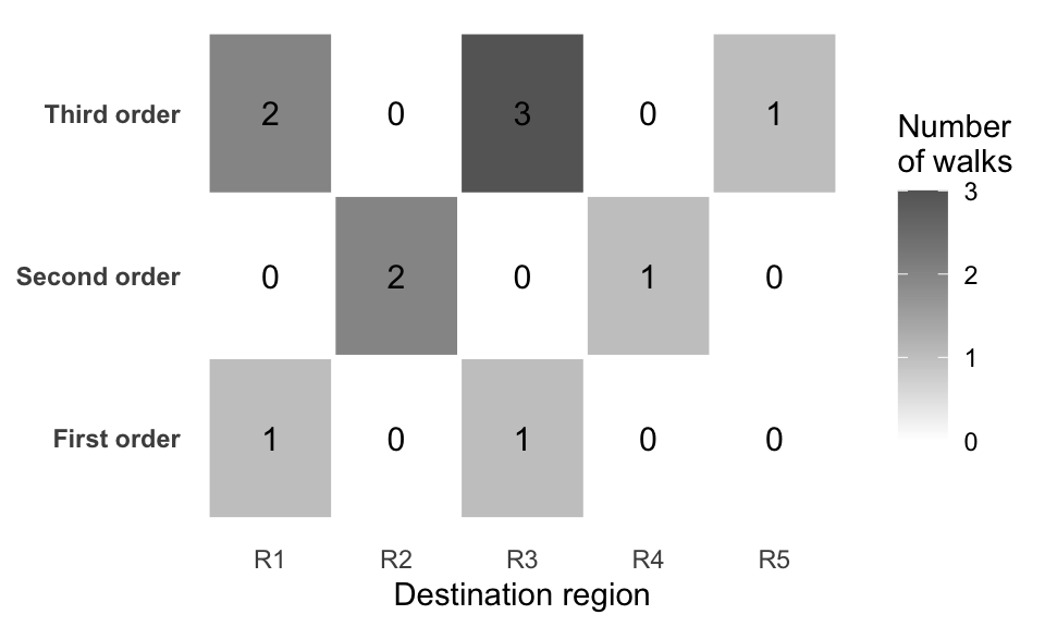
The entries in the figure describe connectivity generated by repeated matrix multiplication. They are not economic effects by themselves. Their econometric meaning depends on the model in which the powers appear. In a spatial autoregressive model, for example, powers of \(\mathbf W\) arise through the spatial multiplier and describe how an initial change can propagate along increasingly long walks. This connection is developed in the following chapters.

1.6 Examples of Spatial Weights Matrices in R

The previous sections introduced several ways to define spatial connections. We now implement those ideas in R using the sf and spdep packages (Pebesma 2018; Bivand et al. 2013).

The objective is to follow the complete sequence \[ \text{spatial data} \longrightarrow \text{neighbors} \longrightarrow \text{weights} \longrightarrow \text{spatially lagged variables}. \]

The example uses the 52 municipalities of the Metropolitan Region of Chile. Each municipality is represented by a polygon, and the order of those polygons will determine the order of the rows and columns in every spatial weights matrix constructed below.

NoteFiles that make up a shapefile

A shapefile usually consists of several files with the same base name. The .shp file stores the geometries, the .dbf file stores the associated variables, and the .shx file stores an index that connects both components. A .prj file commonly records the coordinate reference system. These files should remain together in the same directory.

1.6.1 Reading and Preparing the Spatial Data

We begin by reading the municipal boundaries as an sf object. An sf object combines the geometry of each spatial unit with its associated variables in a single data frame.

The main functions used in the first code block are:

• sf::read_sf(dsn, quiet) reads a spatial data source. The argument dsn gives the file path, while quiet = TRUE suppresses informational messages.
• sf::st_transform(x, crs) changes the coordinate reference system of the spatial object x. Here, crs = 32719 refers to UTM zone 19S, whose coordinates are measured in meters.
• sf::st_point_on_surface(x) creates one representative point inside each polygon. This is useful because the distance-based methods used later require point coordinates.
• sf::st_coordinates(x) extracts the numerical coordinates of those points.

# Read the municipal boundaries.
mr <- sf::read_sf(
  "data/raw/mr_chile/mr_chile.shp",
  quiet = TRUE
)

# Transform the geometries to UTM zone 19S.
mr_projected <- sf::st_transform(
  mr,
  crs = 32719
)

# Construct one representative point inside each municipality.
municipality_points <- sf::st_point_on_surface(
  sf::st_geometry(mr_projected)
)

# Extract the projected coordinates of the representative points.
coords <- sf::st_coordinates(municipality_points)

# Summarize the imported data.
c(
  observations = nrow(mr),
  non_geometry_variables = ncol(sf::st_drop_geometry(mr)),
  geographic_crs = sf::st_crs(mr)$input,
  projected_crs = sf::st_crs(mr_projected)$input
)

          observations non_geometry_variables         geographic_crs 
                  "52"                   "30"               "WGS 84" 
         projected_crs 
          "EPSG:32719" 

The projected coordinates are needed only for methods based on distance. Queen and rook contiguity are determined from the polygon boundaries themselves.

ImportantThe observation order must remain unchanged

The order of the spatial units is part of the definition of the weights matrix. Row \(i\) and column \(i\) must refer to the same municipality as observation \(i\) in the data.

Thus, two objects do not match merely because they contain the same number of municipalities. They must also contain them in the same order. Reordering the data after constructing the neighbors changes the meaning of every row and column of the implied weights matrix.

1.6.2 Creating Contiguity Neighbors

The function spdep::poly2nb() determines which polygons are neighbors. It returns an object of class nb, which is a list with one element for each spatial unit. Element \(i\) contains the numerical indices of the neighbors of unit \(i\).

The main arguments are:

• the first argument is the polygon object;
• queen = TRUE treats polygons that share a border or a corner as neighbors;
• queen = FALSE uses the more restrictive rook criterion;
• row.names = mr$NAME attaches the municipality names to the neighbor list and helps preserve the correspondence with the data.

# Construct queen-contiguity neighbors.
queen_nb <- spdep::poly2nb(
  mr_projected,
  queen = TRUE,
  row.names = mr$NAME
)

# Construct rook-contiguity neighbors.
rook_nb <- spdep::poly2nb(
  mr_projected,
  queen = FALSE,
  row.names = mr$NAME
)

# Verify that the municipality identifiers preserve the data order.
stopifnot(
  identical(
    as.character(attr(queen_nb, "region.id")),
    as.character(mr$NAME)
  ),
  identical(
    as.character(attr(rook_nb, "region.id")),
    as.character(mr$NAME)
  )
)

To understand the object, consider one municipality. The function spdep::card() counts the number of neighbors of every unit. We use which.max() to identify the municipality with the largest queen-neighbor set and then inspect the corresponding element of queen_nb.

# Count queen neighbors for each municipality.
queen_cardinality <- spdep::card(queen_nb)

# Select the municipality with the largest number of queen neighbors.
max_queen_index <- which.max(queen_cardinality)

# Display the focal municipality and the names of its queen neighbors.
list(
  focal_municipality = mr$NAME[max_queen_index],
  number_of_neighbors = queen_cardinality[max_queen_index],
  neighbors = mr$NAME[queen_nb[[max_queen_index]]]
)

$focal_municipality
[1] "San Bernardo"

$number_of_neighbors
[1] 12

$neighbors
 [1] "Cerillos"        "El Bosque"       "La Cisterna"     "La Pintana"     
 [5] "Lo Espejo"       "Puente Alto"     "Maipu"           "Pirque"         
 [9] "Buin"            "Calera de Tango" "Talagante"       "Isla de Maipo"  

The expression

queen_nb[[max_queen_index]]

extracts the neighbor indices stored for the selected municipality. These indices can be used to recover the corresponding municipality names or to highlight them on a map.

Figure 1.7: Municipality with the largest queen-neighbor set

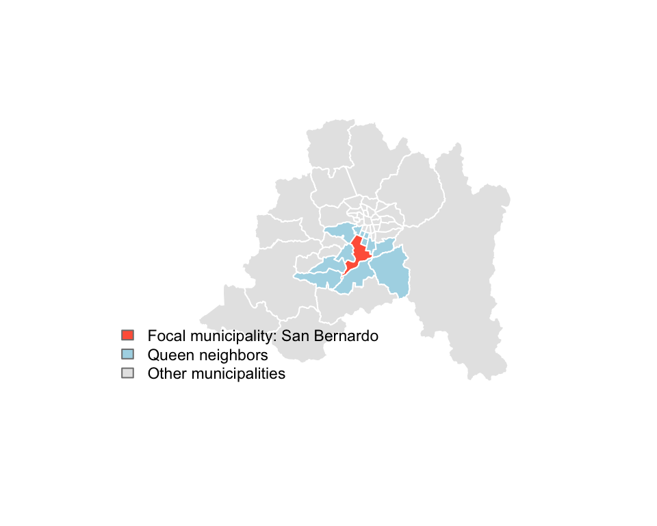
The map provides a direct interpretation of the nb object: the highlighted municipalities are precisely the indices stored in the neighbor list for the focal unit.

1.6.2.1 Diagnosing the Neighbor Structure

Before converting neighbors into weights, it is useful to inspect the structure that has been created.

The functions used below are:

• spdep::card(nb) returns the number of neighbors of each unit;
• spdep::n.comp.nb(nb) identifies the connected components of the neighbor structure; its element $nc gives their number.

An isolate has zero neighbors. A network may have no isolates and still contain several disconnected groups, so both properties should be checked.

# Count the neighbors under each contiguity criterion.
queen_cardinality <- spdep::card(queen_nb)
rook_cardinality  <- spdep::card(rook_nb)

# Identify municipalities with no neighbors.
queen_isolates <- which(queen_cardinality == 0)
rook_isolates  <- which(rook_cardinality == 0)

# Count the connected components.
queen_components <- spdep::n.comp.nb(queen_nb)$nc
rook_components  <- spdep::n.comp.nb(rook_nb)$nc

Table 1.1 reports the statistics most useful for diagnosing the two neighbor definitions.

Table 1.1: Summary of queen and rook contiguity neighbors

Criterion	Average neighbors	Minimum neighbors	Maximum neighbors	Isolates	Connected components
Queen	5.62	2	12	0	1
Rook	5.23	2	10	0	1

Queen contiguity typically produces at least as many neighbors as rook contiguity because it includes both border and corner contacts. The diagnostics show whether that general expectation holds in the current data and whether either rule produces isolates or disconnected groups.

1.6.3 Converting Neighbors into Spatial Weights

An nb object records only which units are neighbors. To use those connections in matrix calculations, we convert the neighbor list into a listw object with spdep::nb2listw().

The principal arguments are:

• the first argument is the neighbor list;
• style = "W" applies row standardization, so the weights in every nonzero row sum to one;
• zero.policy = FALSE requests an error if a unit has no neighbors. This is appropriate here because the diagnostics have already confirmed that there are no isolates.

# Confirm that row standardization is defined for every municipality.
stopifnot(
  length(queen_isolates) == 0,
  length(rook_isolates) == 0
)

# Convert the neighbor lists into row-standardized weights.
queen_lw <- spdep::nb2listw(
  queen_nb,
  style = "W",
  zero.policy = FALSE
)

rook_lw <- spdep::nb2listw(
  rook_nb,
  style = "W",
  zero.policy = FALSE
)

For binary queen weights, a municipality with \(m_i\) neighbors assigns weight \(w_{ij}=\frac{1}{m_i}\) to each of them. Thus, the neighbor list determines which municipalities receive positive weight, while style = "W" determines how the total row weight is distributed among them.

The reciprocal nature of queen and rook contiguity does not imply that the row-standardized numerical weights are symmetric. If municipality \(i\) has two neighbors and municipality \(j\) has five, then a reciprocal connection may satisfy \[ w_{ij}=\frac12, \qquad w_{ji}=\frac15. \]

The function spdep::is.symmetric.nb() checks whether the neighbor relation is reciprocal. The function spdep::listw2mat() converts a listw object into an ordinary numerical matrix, which allows us to compare that matrix with its transpose.

Table 1.2: Symmetry before and after row standardization

Criterion	Neighbor relation symmetric	Row-standardized matrix symmetric
Queen	TRUE	FALSE
Rook	TRUE	FALSE

NoteOther coding schemes in spdep

The argument style in nb2listw() can apply several coding schemes. The most common options include:

• "B": retain binary weights;
• "W": make each nonzero row sum to one;
• "C": scale all weights so that their total equals (n);
• "U": scale all weights so that their total equals one;
• "S": apply a variance-stabilizing transformation;
• "minmax": scale using the maximum row and column sums.

The examples in this chapter use "W" because the objective is to work with row-standardized weights. Changing style changes the numerical meaning and scale of the resulting spatially weighted variables; it is therefore a modeling decision, not merely a software option.

Figure 1.8 compares the queen and rook neighbor structures. The lines are drawn between the representative points of connected municipalities; the polygons remain visible in the background.

Figure 1.8: Queen (left) and rook (right) contiguity networks

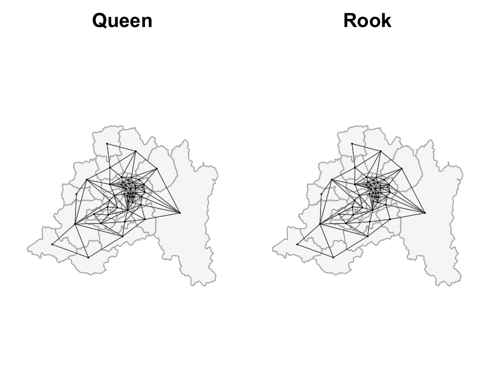
1.6.4 Creating Distance-Based Neighbors

Contiguity uses polygon boundaries. Distance-based rules instead use the coordinates in coords, which are expressed in meters because the data were projected to UTM zone 19S.

We construct two alternatives:

1. \(k\)-nearest-neighbor relations, which keep the number of selected neighbors fixed; and
2. a distance band, which keeps the geographic reach fixed.

1.6.4.1 \(k\)-Nearest Neighbors

The function spdep::knearneigh() identifies the nearest locations.

Its main arguments are:

• the first argument is the coordinate matrix;
• k specifies how many nearest neighbors are selected for each location;
• longlat = FALSE requests planar distances because the coordinates are projected and measured in meters.

The resulting object is converted into an nb neighbor list with spdep::knn2nb(). The argument row.names = mr$NAME attaches the municipality identifiers in the original observation order.

# Identify the one and two nearest municipalities to each location.
knn_1 <- spdep::knearneigh(
  coords,
  k = 1,
  longlat = FALSE
)

knn_2 <- spdep::knearneigh(
  coords,
  k = 2,
  longlat = FALSE
)

# Convert the results into neighbor-list objects.
knn_1_nb <- spdep::knn2nb(
  knn_1,
  row.names = mr$NAME
)

knn_2_nb <- spdep::knn2nb(
  knn_2,
  row.names = mr$NAME
)

A \(k\)-nearest-neighbor relation need not be reciprocal. Municipality \(j\) may be among the \(k\) closest municipalities to \(i\), while \(i\) is not among the \(k\) closest municipalities to \(j\).

The function spdep::make.sym.nb() creates a reciprocal version by retaining a connection whenever either unit selects the other. This changes the original neighbor rule and is shown only for comparison.

Table 1.3: Symmetry of selected nearest-neighbor relations

Relation	Symmetric
1-nearest neighbor	FALSE
2-nearest neighbors	FALSE
Symmetrized 2-nearest neighbors	TRUE

1.6.4.2 Distance-Band Neighbors

A distance band connects all municipalities separated by no more than a selected threshold. To avoid isolates, we use the largest first-nearest-neighbor distance in the sample: \[ d_{\max} = \max_i \left\{ \min_{j\neq i}d_{ij} \right\}. \]

The code proceeds in three steps.

First, spdep::nbdists(nb, coords, longlat) calculates the distances associated with the links in an existing neighbor list. We apply it to the one-nearest- neighbor relation.

Second, the maximum of those distances becomes the threshold.

Third, spdep::dnearneigh() constructs the distance-band relation. Its main arguments are:

• the coordinate matrix;
• d1 and d2, the lower and upper distance limits;
• longlat = FALSE, because the coordinates are projected;
• bounds = c("GT", "LE"), meaning that distances must be greater than d1 and less than or equal to d2;
• row.names = mr$NAME, which preserves the municipality identifiers.

# Calculate each municipality's first-nearest-neighbor distance.
nearest_neighbor_distances <- unlist(
  spdep::nbdists(
    knn_1_nb,
    coords,
    longlat = FALSE
  )
)

# Use the largest of those distances as the distance-band threshold.
maximum_nearest_distance <- max(nearest_neighbor_distances)

# Connect all municipalities whose distance lies in (0, d_max].
distance_band_nb <- spdep::dnearneigh(
  coords,
  d1 = 0,
  d2 = maximum_nearest_distance,
  row.names = mr$NAME,
  longlat = FALSE,
  bounds = c("GT", "LE")
)

# Diagnose isolates and connected components.
distance_band_cardinality <- spdep::card(distance_band_nb)
distance_band_components <- spdep::n.comp.nb(distance_band_nb)$nc

c(
  isolates = sum(distance_band_cardinality == 0),
  connected_components = distance_band_components
)

            isolates connected_components 
                   0                    1 

The chosen threshold guarantees that every municipality reaches at least its closest neighbor. It does not necessarily guarantee that the complete network contains only one connected component, which is why both quantities are reported.

1.6.4.3 Inverse-Distance Weights within the Distance Band

The distance band determines which pairs are connected. We can then replace the binary connections by inverse-distance weights.

The function spdep::nbdists() returns a list whose \(i\)th element contains the distances from municipality \(i\) to the neighbors stored in distance_band_nb. We transform each positive distance \(d_{ij}\) into \(1/d_{ij}\).

The argument glist in spdep::nb2listw() supplies these nonbinary weights. The argument style = "W" then row-standardizes them. Thus, nearby neighbors receive more raw weight, but the final weights in every row still sum to one.

# Calculate the distances associated with the distance-band links.
link_distances <- spdep::nbdists(
  distance_band_nb,
  coords,
  longlat = FALSE
)

# Check that every link distance is finite and strictly positive.
stopifnot(
  all(vapply(
    link_distances,
    function(current_distances) {
      all(is.finite(current_distances) & current_distances > 0)
    },
    logical(1)
  ))
)

# Convert distances into raw inverse-distance weights.
inverse_distance_weights <- lapply(
  link_distances,
  function(current_distances) {
    1 / current_distances
  }
)

# Attach the inverse-distance weights and row-standardize them.
inverse_distance_lw <- spdep::nb2listw(
  distance_band_nb,
  glist = inverse_distance_weights,
  style = "W",
  zero.policy = FALSE
)

Figure 1.9 compares the spatial structures produced by queen contiguity, one-nearest neighbor, two-nearest neighbors, and the distance band.

Figure 1.9: Selected spatial-neighbor schemes for the Metropolitan Region

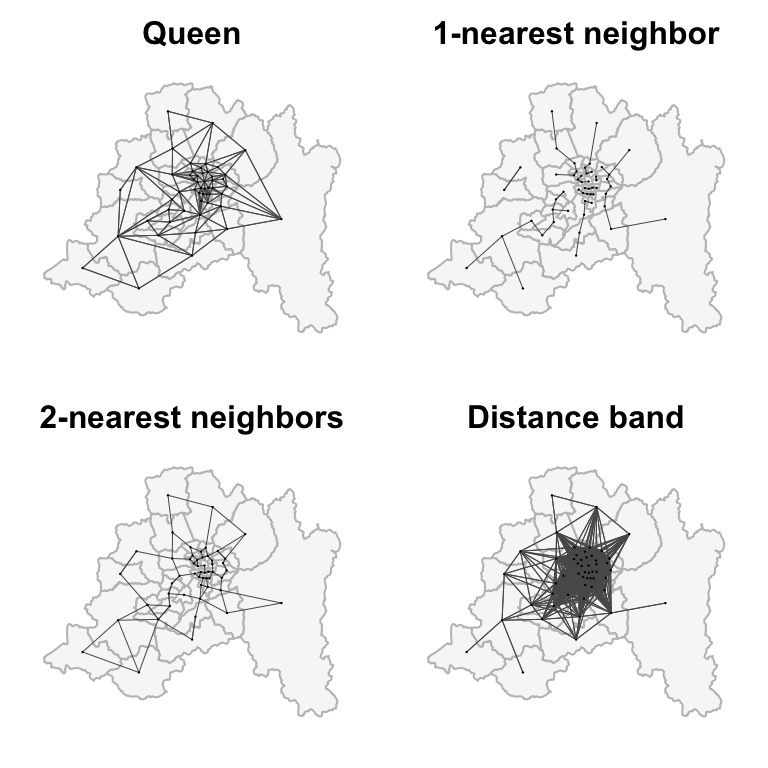
The segments in the figure show which pairs are connected. They do not show the direction of an asymmetric nearest-neighbor relation. Reciprocity must be checked from the nb object rather than inferred from the map.

The four constructions answer different questions:

• queen contiguity asks which polygons touch;
• one- and two-nearest neighbors fix the number of selected neighbors;
• the distance band fixes the maximum geographic reach.

The choice among them should follow the interaction mechanism relevant to the application (Stewart and Zhukov 2010).

1.6.5 Constructing Spatially Lagged Variables in R

The final step is to use a listw object to calculate a spatial lag. The function spdep::lag.listw() evaluates \[ \mathbf W\mathbf y. \]

Its principal arguments are:

• the first argument is the listw object containing the neighbors and weights;
• the second argument is the numerical variable to be spatially lagged;
• zero.policy = FALSE requests an error if a zero-neighbor unit is encountered;
• NAOK = FALSE requests an error if the variable contains missing values.

We use the row-standardized queen weights to construct spatial lags of poverty and urban population.

# Confirm that the variables and the weights object have compatible lengths
# and contain no missing values.
stopifnot(
  length(mr$POVERTY) == length(queen_lw$neighbours),
  length(mr$URB_POP) == length(queen_lw$neighbours),
  !anyNA(mr$POVERTY),
  !anyNA(mr$URB_POP)
)

# Calculate queen row-standardized spatial lags.
mr$W_POVERTY <- spdep::lag.listw(
  queen_lw,
  mr$POVERTY,
  zero.policy = FALSE,
  NAOK = FALSE
)

mr$W_URB_POP <- spdep::lag.listw(
  queen_lw,
  mr$URB_POP,
  zero.policy = FALSE,
  NAOK = FALSE
)

Because queen_lw was constructed with style = "W", W_POVERTY is the average poverty rate among the queen neighbors of each municipality. Likewise, W_URB_POP is the average urban population among those neighbors.

The formula can be verified manually for one municipality. The object

queen_lw$neighbours[[i]]

contains its neighbor indices, while

queen_lw$weights[[i]]

contains the corresponding row-standardized weights.

# Select the first municipality.
i <- 1L

# Calculate its poverty lag directly from its neighbors and weights.
manual_poverty_lag <- sum(
  queen_lw$weights[[i]] *
    mr$POVERTY[queen_lw$neighbours[[i]]]
)

# Verify that the manual calculation agrees with lag.listw().
stopifnot(
  isTRUE(all.equal(
    manual_poverty_lag,
    mr$W_POVERTY[i],
    tolerance = 1e-12
  ))
)

This calculation implements directly \[ (\mathbf W\mathbf y)_i = \sum_{j=1}^{n}w_{ij}y_j. \]

The first six observations are displayed in Table 1.4.

Table 1.4: Observed variables and their queen row-standardized spatial lags

Municipality	Poverty	Queen lag of poverty	Urban population	Queen lag of urban population
Santiago	8	9.10	159919	100138.9
Cerillos	9	12.40	65262	299498.4
Cerro Navia	18	14.00	131850	144756.5
Conchali	12	14.60	104634	121974.2
El Bosque	14	18.25	166514	170266.5
Estacion Central	10	10.43	109573	236231.1

The resulting spatial lag is determined jointly by three choices:

1. the observed variable;
2. the definition of the neighbors; and
3. the coding of the weights.

Changing any of these elements changes the spatially lagged variable.

1.7 Measuring and Testing Global Spatial Autocorrelation

Spatial autocorrelation asks whether values observed in connected spatial units tend to be more similar, or more dissimilar, than would be expected under a specified model of spatial randomness. A global statistic summarizes this association over the entire study region.

The discussion proceeds in two stages. We first use an invented example to develop the intuition behind the Moran scatterplot and Moran’s \(I\). We then introduce the reference models used for statistical inference. All empirical implementation is postponed until the application to municipal poverty in the Metropolitan Region of Chile.

ImportantAssociation is not a mechanism

A statistically significant measure of spatial autocorrelation indicates that the observed spatial arrangement is difficult to reconcile with a stated null model. It does not, by itself, identify why the pattern arose. Similar values may be located near one another because of spatial interaction, common observed characteristics, omitted spatially structured variables, shared shocks, sorting, or other mechanisms.

1.7.1 A Graphical Introduction: The Moran Scatterplot

The Moran scatterplot compares two quantities for every spatial unit: (1) the standardized value observed in that unit; and (2) the spatial lag of the standardized values observed in its neighbors. Let \(x_i\) denote the value observed in unit \(i\). Define its standardized value as \[ z_i = \frac{x_i-\bar{x}}{s_x}, \tag{1.40}\] where \[ \bar{x} = \frac{1}{n} \sum_{i=1}^{n}x_i \] and \(s_x>0\) is a common measure of scale. Let \(\mathbf z=(z_1,\ldots,z_n)^\top\).Given a spatial weights matrix \(\mathbf W\), define \[ \mathbf q = \mathbf W\mathbf z. \tag{1.41}\]

The Moran scatterplot contains the points \[ (z_i,q_i), \qquad i=1,\ldots,n. \tag{1.42}\]

The horizontal coordinate tells us whether unit \(i\) has a value above or below the overall mean. The vertical coordinate tells us whether the weighted values in its spatial neighborhood are, on average, above or below the mean.

Only the original variable is standardized directly. The vertical coordinate is obtained by applying \(\mathbf W\) to the standardized variable. It is not standardized again, because doing so would change the slope of the scatterplot.

The signs of the two coordinates define four descriptive quadrants:

Quadrant	\(z_i\)	\((\mathbf W\mathbf z)_i\)	Interpretation
High–High	\(+\)	\(+\)	An above-average value surrounded by above-average values
Low–High	\(-\)	\(+\)	A below-average value surrounded by above-average values
Low–Low	\(-\)	\(-\)	A below-average value surrounded by below-average values
High–Low	\(+\)	\(-\)	An above-average value surrounded by below-average values

High–High and Low–Low observations display similarity between a unit and its spatial neighborhood. High–Low and Low–High observations display a contrast.

1.7.1.1 An Example

To visualize these ideas, consider 16 artificial spatial units arranged in a regular \(4\times4\) grid. Suppose that the observed values are \[ \begin{pmatrix} 9 & 8 & 2 & 1\\ 8 & 7 & 2 & 1\\ 2 & 2 & 1 & 1\\ 1 & 1 & 1 & 8 \end{pmatrix}. \tag{1.43}\]

The upper-left units form a group of relatively high values, many of the remaining units have relatively low values, and the unit in the lower-right corner has a high value surrounded by low values. We use rook contiguity and row-standardize the resulting binary weights.

Figure 1.10 shows the corresponding Moran scatterplot. The example is entirely artificial and is included only to explain how the graph should be read.

Figure 1.10: Stylized Moran scatterplot for an invented spatial system

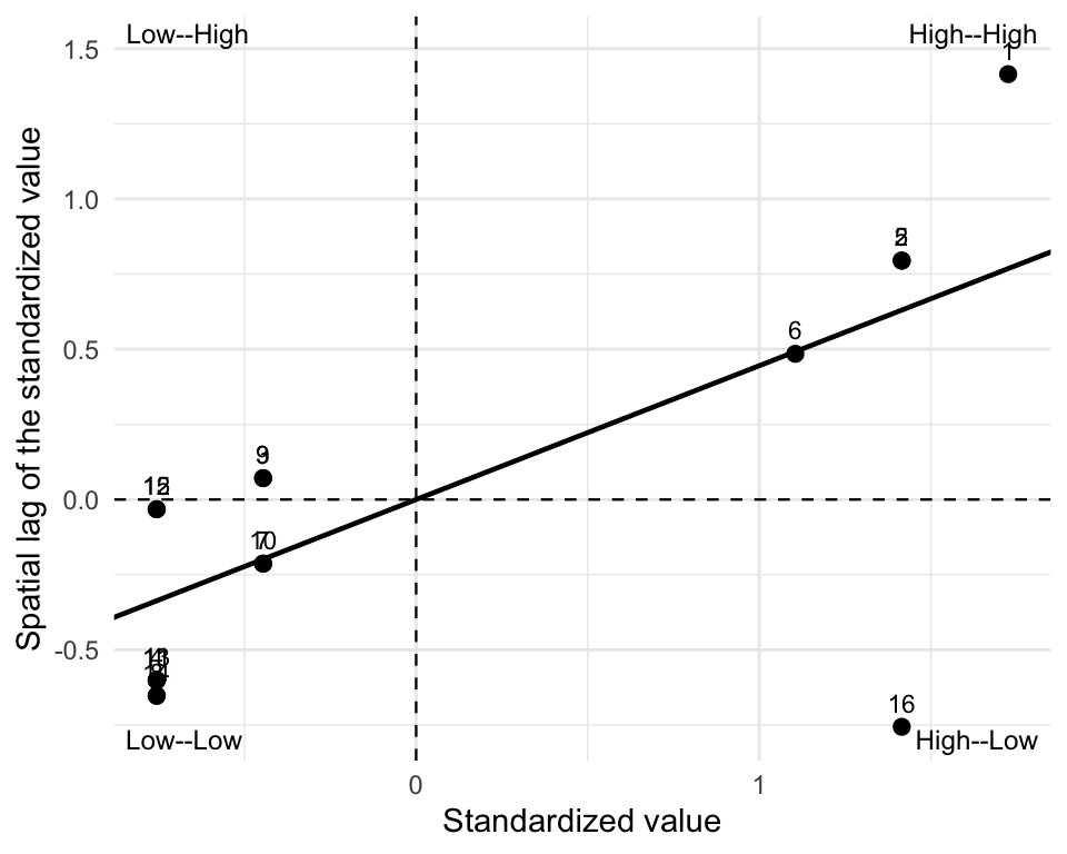
Most of the units in the upper-right and lower-left quadrants reinforce positive spatial association. The high value in the lower-right corner of the invented grid appears in the High–Low quadrant because its surrounding units have low values. Its contribution therefore works against the overall positive pattern. The quadrant assignments are descriptive. They do not constitute tests of local statistical significance.

1.7.2 Global Moran’s \(I\)

The Moran scatterplot suggests how to summarize the global pattern. For each unit, the product \(z_i(\mathbf W\mathbf z)_i\) is positive when the unit and its spatial neighborhood lie on the same side of the mean, and negative when they lie on opposite sides. Summing these products gives \[ \mathbf z^\top\mathbf W\mathbf z = \sum_{i=1}^{n} z_i(\mathbf W\mathbf z)_i. \tag{1.44}\]

Let \[ S_0 = \sum_{i=1}^{n} \sum_{j=1}^{n} w_{ij} \] denote the global sum of weights.

Definition 1.4 (Moran’s \(I\)) For a nonconstant variable \(\mathbf x\) and a spatial weights matrix \(\mathbf W\) satisfying \(S_0>0\), the global Moran statistic is \[ I = \frac{n}{S_0} \frac{ \mathbf z^\top \mathbf W \mathbf z }{ \mathbf z^\top \mathbf z }. \tag{1.45}\]

Equivalently, \[ I = \frac{n}{S_0} \frac{ \displaystyle \sum_{i=1}^{n} \sum_{j=1}^{n} w_{ij}z_i z_j }{ \displaystyle \sum_{i=1}^{n}z_i^2 }. \tag{1.46}\]

If \(\mathbf W\) is row-stochastic and contains no zero rows, then \(S_0=n.\) Moran’s \(I\) then simplifies to \[ I = \frac{ \mathbf z^\top \mathbf W \mathbf z }{ \mathbf z^\top \mathbf z }. \tag{1.47}\]

A positive value indicates that connected units tend to have deviations with the same sign. A negative value indicates that connected units tend to have deviations with opposite signs.

Moran’s \(I\) is not an ordinary Pearson correlation coefficient and is not generally restricted to the interval \([-1,1]\). Its attainable values depend on the spatial weights matrix. Its sign and magnitude describe the observed arrangement, but statistical inference requires a reference distribution.

1.7.3 The Slope of the Moran Scatterplot

The line in the Moran scatterplot is not added merely as a visual aid. Its slope is directly related to Moran’s \(I\).

Proposition 1.2 (Slope of the Moran Scatterplot) Let \(\mathbf z\) be the centered or standardized variable and let \[ \mathbf q = \mathbf W\mathbf z. \]

The ordinary least-squares slope from regressing \(q_i\) on \(z_i\), with or without an intercept, is \[ \widehat\beta = \frac{ \mathbf z^\top\mathbf W\mathbf z }{ \mathbf z^\top\mathbf z } = \frac{S_0}{n}I. \tag{1.48}\]

If \(\mathbf W\) is row-stochastic and contains no zero rows, then \[ \widehat\beta=I. \tag{1.49}\]

Proof. Because \(\mathbf z\) is centered, \(\bar z=\frac{1}{n}\sum_{i=1}^{n}z_i=0.\) Let \(q_i=(\mathbf W\mathbf z)_i\), and denote the sample mean of the spatial lag by \(\bar q\). The OLS slope in a regression with an intercept is \[ \widehat\beta = \frac{ \sum_{i=1}^{n} (z_i-\bar z)(q_i-\bar q) }{ \sum_{i=1}^{n} (z_i-\bar z)^2 }. \]

Using \(\bar z=0\) gives \[ \begin{aligned} \widehat\beta &= \frac{ \sum_{i=1}^{n} z_i(q_i-\bar q) }{ \sum_{i=1}^{n}z_i^2 } \\ &= \frac{ \sum_{i=1}^{n}z_iq_i - \bar q\sum_{i=1}^{n}z_i }{ \sum_{i=1}^{n}z_i^2 } \\ &= \frac{ \sum_{i=1}^{n}z_iq_i }{ \sum_{i=1}^{n}z_i^2 } \\ &= \frac{ \mathbf z^\top\mathbf W\mathbf z }{ \mathbf z^\top\mathbf z }. \end{aligned} \]

The slope from a regression constrained to pass through the origin is the same ratio. Finally, rearranging Equation 1.45 gives \[ \frac{ \mathbf z^\top\mathbf W\mathbf z }{ \mathbf z^\top\mathbf z } = \frac{S_0}{n}I. \]

If \(S_0=n\), the slope equals Moran’s \(I\).

The regression with an intercept generally has \(\widehat\alpha=\overline{\mathbf W\mathbf z}\), which need not equal zero. Nevertheless, allowing an intercept does not change the slope because the horizontal variable is centered. The line through the origin is the conventional reference line shown in the Moran scatterplot.

1.7.4 What Moran’s \(I\) Does and Does Not Measure

Moran’s \(I\) is a global summary. It combines all the products \(z_i(\mathbf W\mathbf z)_i\) into a single statistic. A positive global value may coexist with individual High–Low or Low–High observations, as the invented example illustrates.

The statistic does not identify:

• which units form statistically significant local clusters;
• which observations are statistically significant spatial outliers;
• whether the pattern is causal; or
• which economic, social, environmental, or institutional mechanism generated it.

Those questions require additional models or local statistics.

1.7.5 Reference Models for Spatial Randomness

Calculating Moran’s \(I\) describes the observed spatial arrangement. Deciding whether that value is unusual requires a probability model describing what would count as spatial randomness.

Two classical reference models are commonly used:

Reference model	What is treated as random?	What remains fixed?
Normality	New independent values are generated	The locations and \(\mathbf W\)
Randomization	The observed values are reassigned across locations	The set of observed values and \(\mathbf W\)

1.7.5.1 Normality Reference Model

Under the normality model, \[ x_i \overset{\mathrm{iid}}{\sim} \mathcal N(\mu,\sigma^2). \]

The null hypothesis imagines repeated samples of independent normal observations. Both the numerical values and their realized allocation across the spatial units vary across hypothetical samples.

1.7.5.2 Randomization Reference Model

Under randomization, the observed numerical values are held fixed. Their assignment to the spatial units is treated as exchangeable. The null distribution is generated by reallocating the same observed values while holding \(\mathbf W\) fixed.

For an upper-tail test of positive spatial autocorrelation, the hypotheses can be expressed as \[ H_0: \text{the observed arrangement follows the selected reference model} \] against \[ H_1: \text{Moran's $I$ is unusually large under that reference model}. \]

A lower-tail alternative examines negative spatial autocorrelation, while a two-sided alternative examines unusually large departures in either direction.

Both classical reference models imply \[ \mathbb E_0(I) = -\frac{1}{n-1}. \tag{1.50}\]

The finite-sample expectation is therefore slightly negative rather than zero. Centering imposes the restriction \[ \sum_{i=1}^{n}z_i=0, \] which creates a small negative dependence among the centered observations. The null expectation approaches zero as the number of spatial units increases.

1.7.6 Analytical Inference

Analytical tests standardize the observed statistic as \[ Z_I = \frac{ I-\mathbb E_0(I) }{ \sqrt{\operatorname{Var}_0(I)} }. \tag{1.51}\]

Under suitable regularity conditions, \(Z_I\) is compared with a standard normal distribution. This comparison is an approximation and is not generally an exact finite-sample result.

To state the analytical variances, define \[ S_1 = \frac{1}{2} \sum_{i=1}^{n} \sum_{j=1}^{n} (w_{ij}+w_{ji})^2, \tag{1.52}\] and \[ S_2 = \sum_{i=1}^{n} (w_{i\cdot}+w_{\cdot i})^2, \tag{1.53}\] where \(w_{i\cdot}=\sum_{j=1}^{n}w_{ij}\) and \(w_{\cdot i}=\sum_{j=1}^{n}w_{ji}\). These quantities depend on the selected spatial weights matrix. In particular, they account for both row and column weights and remain well defined when a row-standardized matrix is numerically asymmetric.

The following moments are the classical results associated with Moran’s statistic (Cliff and Ord 1973).

Theorem 1.2 (Moran’s \(I\) Under Normality) Suppose that \(x_1,\ldots,x_n\) are independent normal random variables with a common mean and variance, and assume \(n\geq4\). Then \[ \mathbb E_0(I) = -\frac{1}{n-1}, \] and \[ \mathbb E_0(I^2) = \frac{ n^2S_1-nS_2+3S_0^2 }{ S_0^2(n^2-1) }. \tag{1.54}\]

Consequently, \[ \operatorname{Var}_0(I) = \mathbb E_0(I^2) - [\mathbb E_0(I)]^2. \tag{1.55}\]

Under randomization, define \[ b_2 = \frac{ n\displaystyle\sum_{i=1}^{n}z_i^4 }{ \left( \displaystyle\sum_{i=1}^{n}z_i^2 \right)^2 }. \tag{1.56}\]

The quantity \(b_2\) depends on the shape of the observed distribution and enters the randomization variance because the values themselves are held fixed.

Theorem 1.3 (Moran’s \(I\) Under Randomization) Under random assignment of the observed values to the \(n\) locations, with \(n\geq4\), \[ \mathbb E_0(I) = -\frac{1}{n-1}, \] and \[ \mathbb E_0(I^2) = \frac{ \begin{aligned} &n\left[ (n^2-3n+3)S_1 -nS_2 +3S_0^2 \right] \\ &\quad{} -b_2\left[ (n^2-n)S_1 -2nS_2 +6S_0^2 \right] \end{aligned} }{ (n-1)(n-2)(n-3)S_0^2 }. \tag{1.57}\]

Consequently, \[ \operatorname{Var}_0(I) = \mathbb E_0(I^2) - [\mathbb E_0(I)]^2. \tag{1.58}\]

The observed Moran statistic and its null expectation are the same under the two reference models. What changes is the null variance and, consequently, the standardized statistic and p-value.

1.7.7 Permutation Inference

A permutation test implements the randomization model directly. Let \(I_{\mathrm{obs}}\) denote Moran’s statistic for the observed allocation. For each replication \(s=1,\ldots,S\), the observed values are randomly reassigned across the spatial units while \(\mathbf W\) remains fixed, producing a permuted statistic \(I_s^*\).

The procedure is:

1. Calculate \(I_{\mathrm{obs}}\) from the observed allocation.
2. Randomly permute the values across the spatial units.
3. Calculate Moran’s \(I\) for the permuted allocation.
4. Repeat Steps 2 and 3 a total of \(S\) times.
5. Compare the observed statistic with the permutation distribution.

For an upper-tail test, the Monte Carlo p-value is \[ \widehat p = \frac{ 1+ \displaystyle\sum_{s=1}^{S} \mathbf 1\{I_s^*\geq I_{\mathrm{obs}}\} }{ S+1 }. \tag{1.59}\]

Adding one to the numerator and denominator includes the observed allocation among the reference arrangements and prevents a reported p-value of zero.

If all possible reallocations were enumerated, the resulting distribution would be the exact randomization distribution. In realistic applications, the number of allocations is usually too large, so a Monte Carlo test uses a random sample of permutations.

With \(S=999\), the smallest attainable one-sided p-value is \[ \frac{1}{999+1} = 0.001. \]

The next section implements the Moran scatterplot, analytical tests, and permutation inference with the municipal poverty data.

1.8 Application: Poverty in the Metropolitan Region of Chile

This application brings together the tools developed in the chapter. We first map the poverty variable, then construct its empirical Moran scatterplot, perform analytical and permutation tests under queen contiguity, and finally examine robustness to rook contiguity.

The exercise is descriptive rather than causal. A spatial pattern can motivate further investigation, but it does not identify the mechanism that generated it.

1.8.1 Preparing and Mapping the Poverty Data

We begin by creating a named numerical vector. The names are important because they allow spdep to check that the observations follow the same order as the spatial weights object.

poverty_values <- stats::setNames(
  as.numeric(mr$POVERTY),
  as.character(mr$NAME)
)

stopifnot(
  length(poverty_values) == nrow(mr),
  !anyNA(poverty_values),
  all(is.finite(poverty_values)),
  stats::sd(poverty_values) > 0,
  identical(
    names(poverty_values),
    as.character(attr(queen_lw$neighbours, "region.id"))
  )
)

The function stats::setNames() attaches the municipality identifiers to the numeric values. The remaining checks confirm that the variable is complete, finite, nonconstant, and correctly aligned with the queen weights.

A choropleth map provides a first view of the geographic distribution. The map uses five quantile classes, which place approximately the same number of municipalities in each group.

poverty_breaks <- unique(
  stats::quantile(
    poverty_values,
    probs = seq(0, 1, length.out = 6),
    na.rm = TRUE,
    type = 7
  )
)

if (length(poverty_breaks) != 6L) {
  stop(
    paste(
      "The five-class quantile map requires six distinct break points.",
      "Use fewer classes or another classification rule when ties prevent this."
    )
  )
}

mr$poverty_quantile <- cut(
  poverty_values,
  breaks = poverty_breaks,
  include.lowest = TRUE,
  ordered_result = TRUE,
  dig.lab = 4
)

ggplot2::ggplot(mr) +
  ggplot2::geom_sf(
    ggplot2::aes(fill = poverty_quantile),
    color = "white",
    linewidth = 0.2
  ) +
  ggplot2::scale_fill_viridis_d(
    name = "Poverty\nquantile",
    direction = -1,
    drop = FALSE
  ) +
  ggplot2::labs(x = NULL, y = NULL) +
  ggplot2::theme_minimal() +
  ggplot2::theme(
    axis.text = ggplot2::element_blank(),
    axis.ticks = ggplot2::element_blank(),
    panel.grid = ggplot2::element_blank(),
    legend.position = "right"
  )

Figure 1.11: Quantile map of municipal poverty in the Metropolitan Region of Chile

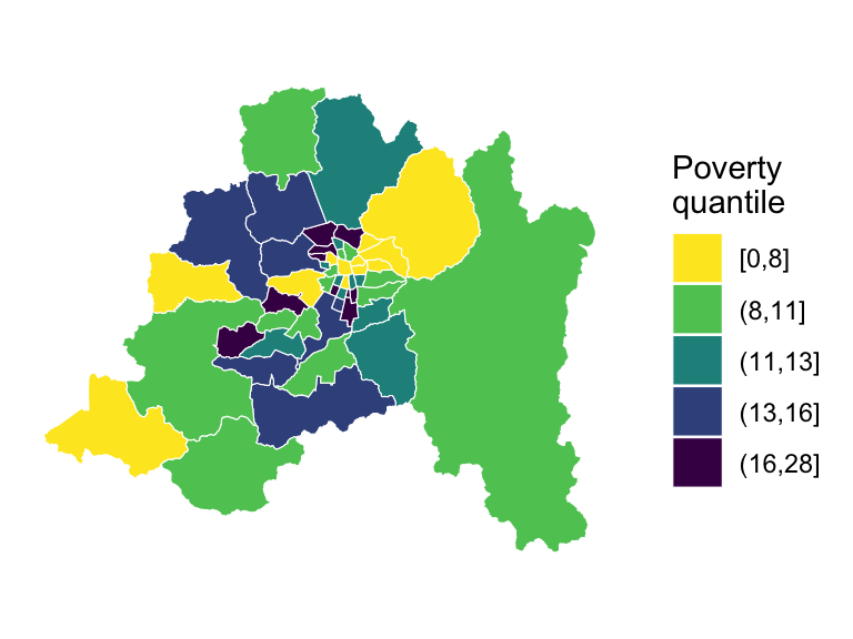
Quantile classes describe relative position within the observed sample. Their boundaries are sample-dependent and should not be interpreted as official or economically meaningful poverty thresholds.

1.8.2 Moran Scatterplot for Municipal Poverty

The empirical Moran scatterplot requires three calculations:

1. scale() centers and standardizes the poverty variable;
2. spdep::lag.listw() computes the spatial lag using the queen weights; and
3. spdep::moran() calculates the observed global Moran statistic.

The principal arguments of spdep::moran() are:

• x: the numerical variable;
• listw: the spatial weights object;
• n: the number of observations;
• S0: the global sum of weights;
• zero.policy = FALSE: request an error if an isolate is encountered; and
• NAOK = FALSE: request an error if the variable contains missing values.

# Standardize poverty once.
poverty_z <- as.numeric(
  scale(poverty_values)
)
names(poverty_z) <- names(poverty_values)

# Calculate the spatial lag of standardized poverty.
poverty_wz <- spdep::lag.listw(
  queen_lw,
  poverty_z,
  zero.policy = FALSE,
  NAOK = FALSE
)

# Calculate the observed Moran statistic.
poverty_moran_components <- spdep::moran(
  poverty_values,
  queen_lw,
  n = length(poverty_values),
  S0 = spdep::Szero(queen_lw),
  zero.policy = FALSE,
  NAOK = FALSE
)

poverty_moran_i <- unname(
  poverty_moran_components$I
)

poverty_moran_plot_data <- data.frame(
  municipality = names(poverty_values),
  z = poverty_z,
  wz = poverty_wz,
  row.names = NULL
)

# Verify that the fitted slope equals Moran's I.
poverty_moran_fit <- stats::lm(
  wz ~ z,
  data = poverty_moran_plot_data
)

stopifnot(
  isTRUE(all.equal(
    unname(stats::coef(poverty_moran_fit)[["z"]]),
    poverty_moran_i,
    tolerance = 1e-10
  ))
)

ggplot2::ggplot(
  poverty_moran_plot_data,
  ggplot2::aes(x = z, y = wz)
) +
  ggplot2::geom_hline(
    yintercept = 0,
    linewidth = 0.4,
    linetype = "dashed"
  ) +
  ggplot2::geom_vline(
    xintercept = 0,
    linewidth = 0.4,
    linetype = "dashed"
  ) +
  ggplot2::geom_point(size = 2) +
  ggplot2::geom_abline(
    intercept = 0,
    slope = poverty_moran_i,
    linewidth = 0.8
  ) +
  ggplot2::annotate(
    "text",
    x = Inf,
    y = Inf,
    label = "High--High",
    hjust = 1.1,
    vjust = 1.4,
    size = 3.2
  ) +
  ggplot2::annotate(
    "text",
    x = -Inf,
    y = Inf,
    label = "Low--High",
    hjust = -0.1,
    vjust = 1.4,
    size = 3.2
  ) +
  ggplot2::annotate(
    "text",
    x = -Inf,
    y = -Inf,
    label = "Low--Low",
    hjust = -0.1,
    vjust = -0.6,
    size = 3.2
  ) +
  ggplot2::annotate(
    "text",
    x = Inf,
    y = -Inf,
    label = "High--Low",
    hjust = 1.1,
    vjust = -0.6,
    size = 3.2
  ) +
  ggplot2::labs(
    x = "Standardized poverty",
    y = "Spatial lag of standardized poverty"
  ) +
  ggplot2::theme_minimal()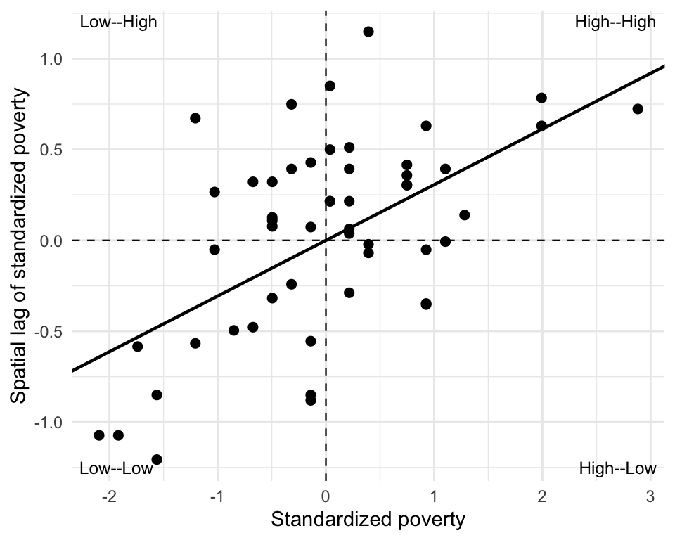

Figure 1.12: Moran scatterplot for municipal poverty

Because queen_lw is row-standardized, the slope of the reference line is the observed Moran statistic. The scatterplot also reveals individual municipalities whose signs differ from those of their spatial neighborhoods, but those quadrant positions are descriptive rather than inferential.

1.8.3 Analytical Inference under Queen Contiguity

The function spdep::moran.test() calculates an analytical Moran test. Its main arguments are:

• x: the observed variable;
• listw: the spatial weights object;
• randomisation = TRUE: use the randomization variance;
• randomisation = FALSE: use the normality variance;
• alternative = "greater": use an upper-tail test for positive spatial autocorrelation;
• zero.policy = FALSE: request an error if an isolate is encountered;
• na.action = stats::na.fail: request an error if the variable contains missing values; and
• spChk = TRUE: check the correspondence between the observation identifiers and the weights object.

Both tests below use exactly the same observed values and row-standardized queen weights. Only the analytical reference variance changes.

queen_moran_randomization <- spdep::moran.test(
  poverty_values,
  queen_lw,
  randomisation = TRUE,
  alternative = "greater",
  zero.policy = FALSE,
  na.action = stats::na.fail,
  spChk = TRUE
)

queen_moran_normality <- spdep::moran.test(
  poverty_values,
  queen_lw,
  randomisation = FALSE,
  alternative = "greater",
  zero.policy = FALSE,
  na.action = stats::na.fail,
  spChk = TRUE
)

extract_moran_test <- function(
  test_object,
  reference_model
) {
  data.frame(
    `Reference model` = reference_model,
    `Observed I` = unname(test_object$estimate[[1]]),
    `Null expectation` = unname(test_object$estimate[[2]]),
    `Null variance` = unname(test_object$estimate[[3]]),
    `Standard deviate` = unname(test_object$statistic),
    `p-value` = format.pval(
      test_object$p.value,
      digits = 4,
      eps = 1e-4
    ),
    check.names = FALSE
  )
}

queen_analytical_results <- rbind(
  extract_moran_test(
    queen_moran_randomization,
    "Randomization"
  ),
  extract_moran_test(
    queen_moran_normality,
    "Normality"
  )
)

knitr::kable(
  queen_analytical_results,
  digits = 4,
  row.names = FALSE
)

Table 1.5: Analytical Moran tests for poverty under queen contiguity

Reference model	Observed I	Null expectation	Null variance	Standard deviate	p-value
Randomization	0.3065	-0.0196	0.0064	4.0689	< 1e-04
Normality	0.3065	-0.0196	0.0065	4.0453	< 1e-04

The observed Moran statistic and its null expectation are the same in both rows. The null variance, standardized deviate, and p-value differ because the reference models make different probabilistic assumptions.

1.8.4 Permutation Inference under Queen Contiguity

The function spdep::moran.mc() performs a Monte Carlo permutation test. Its principal arguments are:

• x: the observed variable;
• listw: the weights matrix, which remains fixed across permutations;
• nsim = 999: generate 999 random reallocations;
• alternative = "greater": use an upper-tail test;
• zero.policy = FALSE: request an error if an isolate is encountered; and
• na.action = stats::na.fail: request an error if values are missing.

The call to set.seed() ensures that the same random permutations can be reproduced.

set.seed(20260715)

n_permutations <- 999L

queen_moran_permutation <- spdep::moran.mc(
  poverty_values,
  queen_lw,
  nsim = n_permutations,
  alternative = "greater",
  zero.policy = FALSE,
  na.action = stats::na.fail
)

queen_moran_permutation

    Monte-Carlo simulation of Moran I

data:  poverty_values 
weights: queen_lw  
number of simulations + 1: 1000 

statistic = 0.3065, observed rank = 1000, p-value = 0.001
alternative hypothesis: greater

Figure 1.13 shows the empirical reference distribution. The vertical line marks the observed statistic.

Figure 1.13: Permutation distribution of Moran’s I under queen contiguity

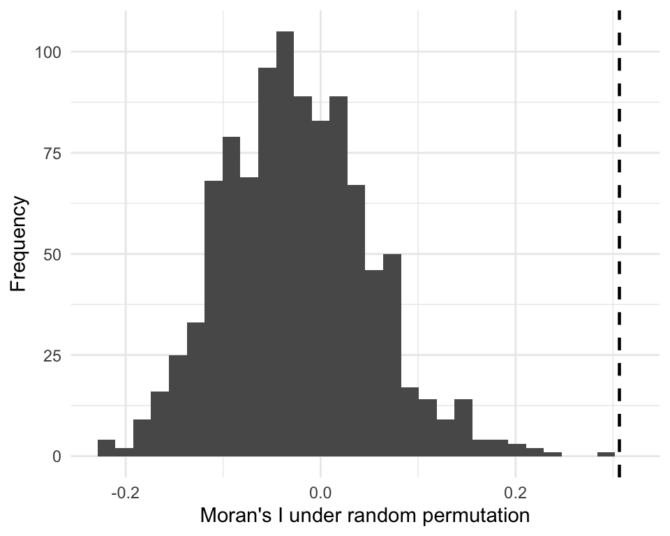
With 999 permutations, the smallest attainable corrected p-value is

\[ \frac{1}{999+1} = 0.001. \]

The p-value should therefore never be reported as zero.

1.8.5 Robustness to Rook Contiguity

Queen and rook contiguity represent different hypotheses about which municipalities are connected. To assess whether the main conclusion depends entirely on the queen criterion, we repeat the randomization-based analytical test and the permutation test using the row-standardized rook weights.

rook_moran_randomization <- spdep::moran.test(
  poverty_values,
  rook_lw,
  randomisation = TRUE,
  alternative = "greater",
  zero.policy = FALSE,
  na.action = stats::na.fail,
  spChk = TRUE
)

set.seed(20260715)

rook_moran_permutation <- spdep::moran.mc(
  poverty_values,
  rook_lw,
  nsim = n_permutations,
  alternative = "greater",
  zero.policy = FALSE,
  na.action = stats::na.fail
)

moran_robustness_results <- data.frame(
  `Weights` = c("Queen", "Rook"),
  `Observed I` = c(
    unname(queen_moran_randomization$estimate[[1]]),
    unname(rook_moran_randomization$estimate[[1]])
  ),
  `Analytical p-value` = format.pval(
    c(
      queen_moran_randomization$p.value,
      rook_moran_randomization$p.value
    ),
    digits = 4,
    eps = 1e-4
  ),
  `Permutation p-value` = format.pval(
    c(
      queen_moran_permutation$p.value,
      rook_moran_permutation$p.value
    ),
    digits = 4,
    eps = 1e-4
  ),
  check.names = FALSE
)

knitr::kable(
  moran_robustness_results,
  digits = 4,
  row.names = FALSE
)

Table 1.6: Moran tests under queen and rook contiguity

Weights	Observed I	Analytical p-value	Permutation p-value
Queen	0.3065	< 1e-04	0.001
Rook	0.3423	< 1e-04	0.001

Changing from queen to rook modifies both the observed statistic and its reference distribution because it changes the spatial connections represented by \(\mathbf W\). Robustness across these two matrices is informative because both are plausible boundary-based definitions. It does not imply robustness to every possible spatial weights specification.

1.8.6 Moran Scatterplot Quadrants

The empirical Moran scatterplot also permits a descriptive classification of the municipalities according to the signs of their standardized poverty values and spatial lags.

poverty_quadrant <- ifelse(
  poverty_z >= 0 & poverty_wz >= 0,
  "High--High",
  ifelse(
    poverty_z < 0 & poverty_wz >= 0,
    "Low--High",
    ifelse(
      poverty_z < 0 & poverty_wz < 0,
      "Low--Low",
      "High--Low"
    )
  )
)

quadrant_levels <- c(
  "High--High",
  "Low--High",
  "Low--Low",
  "High--Low"
)

poverty_quadrant_data <- data.frame(
  municipality = names(poverty_values),
  poverty = poverty_values,
  standardized_poverty = poverty_z,
  spatial_lag = poverty_wz,
  quadrant = factor(
    poverty_quadrant,
    levels = quadrant_levels
  ),
  local_cross_product = poverty_z * poverty_wz,
  row.names = NULL
)

poverty_quadrant_summary <- data.frame(
  `Quadrant` = quadrant_levels,
  `Number of municipalities` = as.integer(
    table(
      factor(
        poverty_quadrant_data$quadrant,
        levels = quadrant_levels
      )
    )
  ),
  check.names = FALSE
)

knitr::kable(
  poverty_quadrant_summary,
  row.names = FALSE
)

Table 1.7: Municipalities by Moran scatterplot quadrant

Quadrant	Number of municipalities
High–High	20
Low–High	11
Low–Low	14
High–Low	7

High–High and Low–Low municipalities contribute positively to the numerator of Moran’s \(I\). High–Low and Low–High municipalities contribute negatively and may deserve closer substantive examination.

The municipalities with the most negative cross-products are reported in Table 1.8.

Table 1.8: Municipalities with the most negative Moran cross-products

Municipality	Poverty	Standardized poverty	Spatial lag	Quadrant	Local cross-product
San Miguel	5	-1.206	0.672	Low–High	-0.811
Padre Hurtado	17	0.926	-0.353	High–Low	-0.327
Huechuraba	17	0.926	-0.347	High–Low	-0.322
Maipu	6	-1.029	0.266	Low–High	-0.274
La Florida	10	-0.318	0.748	Low–High	-0.238

A negative cross-product is not evidence of a statistically significant local outlier. Formal local analysis requires a local indicator of spatial association and careful treatment of the multiple hypotheses examined across municipalities (Anselin 1995).

1.8.7 Main Findings

The exploratory analysis yields four main conclusions:

1. Poverty varies substantially across municipalities in the Metropolitan Region.
2. The empirical Moran scatterplot indicates an overall tendency for municipalities with similar deviations from the mean to be spatially connected.
3. Analytical and permutation tests support positive global spatial autocorrelation under queen contiguity.
4. The main conclusion remains under rook contiguity, although the numerical statistic and p-values change with the spatial weights matrix.

These results describe the global spatial arrangement of poverty. They do not identify statistically significant local clusters and do not establish the economic or social mechanism that generated the observed pattern.

More generally, every conclusion about spatial autocorrelation is conditional on three elements:

1. the variable being analyzed;
2. the spatial weights matrix; and
3. the null reference model.

A reproducible analysis should document and justify all three, together with the definition, source, and reference year of the data.

1.9 Chapter Summary

This chapter introduced the principal objects used to describe spatial connections and evaluate global spatial autocorrelation in cross-sectional data.

The main conclusions are:

1. Spatial dependence is the broad failure of independence among spatial observations. Direct interaction among outcomes is one possible source, but common environments, omitted spatially structured variables, sorting, and shared shocks may produce dependence as well.

2. Spatial interaction refers to a substantive mechanism through which outcomes or characteristics in one unit affect another. Spatial autocorrelation describes an association between observed values and the connectivity encoded by a spatial weights matrix. Autocorrelation alone does not establish interaction or causality.

3. A spatial weights matrix \(\mathbf W\) is a substantive hypothesis about which units are connected and with what relative intensity. Under the convention used in this book, \(w_{ij}\) measures a connection originating in unit \(j\) and received by unit \(i\).

4. Spatial weights may be based on contiguity, distance, nearest neighbors, flows, or other networks. Rook and queen are the most common polygon-contiguity definitions; bishop contiguity is a more specialized alternative.

5. A matrix may be known and treated as fixed without being economically exogenous. The formation of the network must be considered whenever its connections may depend on unobserved determinants of the outcome.

6. Row standardization transforms each nonzero row to sum to one. This often turns a spatial lag into a weighted average, but it removes variation in the original total connection intensity and is undefined for spatial isolates unless an additional convention is imposed.

7. A row-stochastic matrix has eigenvalue one and spectral radius one. When row standardization is applied to an originally symmetric nonnegative matrix with positive row sums, the resulting matrix is similar to a symmetric matrix and therefore has real eigenvalues.

8. The spatial lag \[ (\mathbf W\mathbf y)_i = \sum_{j=1}^n w_{ij}y_j \] combines values originating in units \(j\) and received by destination unit \(i\). Its interpretation as a sum or average depends on the coding of \(\mathbf W\).

9. The element \((\mathbf W^\ell)_{ij}\) aggregates walks of length \(\ell\) originating in \(j\) and terminating in \(i\). Rows collect walks reaching a destination, columns collect walks emanating from an origin, and positive diagonal elements represent closed walks. They become economic feedback effects only within a model that gives them that interpretation.

10. Moran’s \(I\) measures global spatial autocorrelation relative to a selected \(\mathbf W\). The weighting scheme should be kept fixed when comparing analytical and permutation inference: in this chapter, both procedures use the same row-standardized weights. Analytical inference depends on a stated reference model, while permutation inference evaluates the observed statistic against random reallocations of the fixed observed values.

11. A statistically significant Moran’s \(I\) indicates that the observed spatial arrangement is difficult to reconcile with the chosen null model. It does not determine where significant local clusters occur and does not identify a causal spatial process.

1.10 Exercises

Exercise 1.1 (Circular \(k\)-Ahead and \(k\)-Behind Weights)

A weighting scheme often used in Monte Carlo studies places the spatial units on a circle. Each unit has \(k\) neighbors ahead of it and \(k\) neighbors behind it in the sample ordering. The matrix is row-standardized, so every nonzero element equals \(1/(2k)\).

Suppose that \(n=10\) and \(k=2\).

1. Identify the four neighbors of spatial unit 3.
2. Write the complete third row of the \(10\times10\) row-standardized weights matrix.
3. Explain how the circular convention changes the neighbors of units 1 and 10 relative to a non-circular ordering.
4. Verify that the third row sums to one.
5. Is the matrix symmetric? Explain why.

Exercise 1.2 (Minimum Number of Queen Neighbors) Consider a rectangular checkerboard containing at least three rows and three columns.

1. What is the minimum number of queen neighbors that a spatial unit can have?
2. Which units attain this minimum?
3. What is the maximum number of queen neighbors for an interior unit?
4. Explain how the answers change for rook contiguity.
5. Would row standardization preserve the symmetry of the binary matrix at the boundary? Explain.

Exercise 1.3 (Row Standardization and a Common Scale Factor) Let \(INC_i>0\) denote per capita income in spatial unit \(i\). For \(i\neq j\), define the raw weights

\[ w_{ij}^{*} = \alpha \left[ 1- \frac{|INC_i-INC_j|}{INC_i+INC_j} \right], \qquad \alpha>0, \]

with \(w_{ii}^{*}=0\).

1. Show that \(0\leq w_{ij}^{*}\leq\alpha\).
2. Define the row-standardized weights by \[ w_{ij} = \frac{w_{ij}^{*}} {\displaystyle\sum_{\ell=1}^{n}w_{i\ell}^{*}}. \]
3. Prove that the common factor \(\alpha\) cancels from \(w_{ij}\) whenever the row sum is positive.
4. Interpret the economic meaning of a relatively large value of \(w_{ij}^{*}\).
5. Is the raw matrix symmetric? Is the row-standardized matrix necessarily symmetric? Justify both answers.
6. Discuss why using contemporaneous income to construct \(\mathbf W\) may threaten the exogeneity of the weights in an economic model.

Exercise 1.4 (Unstandardized and Row-Standardized Spatial Lags) Consider the raw binary matrix

\[ \mathbf W^{*} = \begin{pmatrix} 0 & 1 & 1 & 0 \\ 1 & 0 & 1 & 1 \\ 1 & 1 & 0 & 0 \\ 0 & 1 & 0 & 0 \end{pmatrix}, \qquad \mathbf y = \begin{pmatrix} 4 \\ 8 \\ 12 \\ 20 \end{pmatrix}. \]

1. Compute \(\mathbf W^{*}\mathbf y\).
2. Construct the row-standardized matrix \(\mathbf W\).
3. Compute \(\mathbf W\mathbf y\).
4. Interpret the second and fourth elements of both spatial lags using the convention that \(w_{ij}\) represents a connection from \(j\) to \(i\).
5. Explain why the difference between the two spatial lags matters when units have very different numbers of neighbors.
6. Is \(\mathbf W\) symmetric? Explain your answer.

Exercise 1.5 (Higher-Order Spatial Connections) Use the raw matrix \(\mathbf W^{*}\) from Exercise 1.4.

1. Compute \((\mathbf W^{*})^2\).
2. Interpret the element \([(\mathbf W^{*})^2]_{14}\) as the number of two-step walks originating in unit 4 and terminating in unit 1.
3. List the intermediate unit associated with each such walk.
4. Explain why diagonal elements of \((\mathbf W^{*})^2\) may be positive even though \(w_{ii}^{*}=0\).
5. Determine whether a positive element of \((\mathbf W^{*})^2\) necessarily identifies a pure second-order neighbor.
6. Compute \((\mathbf W^{*})^2\mathbf y\) and explain how it differs conceptually from \(\mathbf W^{*}\mathbf y\).

Exercise 1.6 (Expected Moran’s \(I\) Under Gaussian Spatial Independence) Let

\[ \mathbf x \sim \mathcal N \left( \mu\boldsymbol\iota_n, \sigma^2\mathbf I_n \right), \]

and define

\[ \mathbf P = \mathbf I_n - \frac{1}{n} \boldsymbol\iota_n \boldsymbol\iota_n^\top, \qquad \mathbf z = \mathbf P\mathbf x. \]

Let \(\mathbf W\) be a real row-standardized spatial weights matrix with zero diagonal and no spatial isolates. Thus,

\[ \mathbf W\boldsymbol\iota_n = \boldsymbol\iota_n, \qquad S_0=n. \]

The matrix \(\mathbf W\) need not be numerically symmetric. Moran’s statistic is

\[ I = \frac{ \mathbf z^\top \mathbf W \mathbf z }{ \mathbf z^\top\mathbf z }. \]

Complete the following steps.

1. Show that \(\mathbf P\) is symmetric and idempotent.
2. Show that \[ \operatorname{tr}(\mathbf P)=n-1. \]
3. Let \(\mathbf Q\) be an \(n\times(n-1)\) matrix whose columns form an orthonormal basis for the range of \(\mathbf P\). Show that \[ \mathbf P = \mathbf Q\mathbf Q^\top. \]
4. Show that there exists a random vector \(\mathbf u\sim\mathcal N(\mathbf0,\mathbf I_{n-1})\) such that \[ \mathbf z = \sigma\mathbf Q\mathbf u. \]
5. Use spherical symmetry to establish \[ \mathbb E \left[ \frac{ \mathbf u\mathbf u^\top }{ \mathbf u^\top\mathbf u } \right] = \frac{1}{n-1}\mathbf I_{n-1}. \]
6. Deduce, without imposing symmetry on \(\mathbf W\), that \[ \mathbb E \left[ \frac{ \mathbf z^\top \mathbf W \mathbf z }{ \mathbf z^\top\mathbf z } \right] = \frac{ \operatorname{tr}(\mathbf W\mathbf P) }{n-1}. \]
7. Use the zero diagonal and row standardization to show that \[ \begin{aligned} \operatorname{tr}(\mathbf W\mathbf P) &= \operatorname{tr}(\mathbf W) - \frac{1}{n} \boldsymbol\iota_n^\top \mathbf W \boldsymbol\iota_n\\ &= 0- \frac{1}{n} \boldsymbol\iota_n^\top \boldsymbol\iota_n\\ &= -1. \end{aligned} \]
8. Conclude that \[ \mathbb E(I) = -\frac{1}{n-1}. \]
9. Verify the result by simulation for at least two values of \(n\) using row-standardized matrices that are not numerically symmetric.

Exercise 1.7 (Applied Exercise: Crime in Columbus) Use the Columbus data included in the spData package.

columbus <- sf::st_read(
  system.file(
    "shapes/columbus.gpkg",
    package = "spData"
  ),
  quiet = TRUE
)

Complete the following analysis.

1. Document the definition and source of the CRIME variable.
2. Plot a choropleth map of CRIME and describe the visible spatial pattern.
3. Construct queen and rook contiguity neighbor lists using spdep::poly2nb().
4. Verify observation-order alignment, spatial isolates, and connected components.
5. Compare the distributions of the number of neighbors under the two criteria.
6. Construct row-standardized listw objects for both criteria.
7. Compute Moran’s \(I\) for CRIME using spdep::moran.test() under the randomization and normality reference models, using the row-standardized queen and rook weights directly.
8. Repeat the analysis using spdep::moran.mc() with 999 permutations and the same row-standardized weights.
9. Construct Moran scatterplots for the queen and rook specifications by standardizing CRIME once and then calculating its spatial lag.
10. Compare the statistics, reference distributions, and conclusions across the two definitions of spatial proximity.
11. Explain whether the substantive conclusion is robust to the choice of \(\mathbf W\) and why neither test establishes a causal mechanism.

Exercise 1.8 (Programming Exercise: A Moran Scatterplot Function) Write an R function called moran_scatterplot() that receives:

• a numeric vector x;
• a spatial weights object listw;
• an optional plot title; and
• a logical option standardize.

The function must:

1. check that the length and ordering of x are compatible with listw;
2. reject missing or non-finite observations with an informative error;
3. when standardize = TRUE, standardize x once and then compute the spatial lag of the resulting vector;
4. when standardize = FALSE, compute the spatial lag of the original vector;
5. produce a scatterplot of the selected horizontal-axis variable against its spatial lag;
6. add horizontal and vertical lines through zero when standardized values are used;
7. add the least-squares regression line;
8. report the fitted slope and intercept; and
9. identify the four Moran scatterplot quadrants when standardized values are used.

Demonstrate the function using:

1. simulated spatially independent data;
2. simulated data with positive spatial autocorrelation; and
3. the CRIME variable from the Columbus data.

For the standardized version, verify that

\[ \widehat\beta = \frac{S_0}{n}I, \]

where \(\widehat\beta\) is the OLS slope. Explain why \(\widehat\beta=I\) when the weights are row-standardized and contain no isolates. Do not standardize the spatial lag a second time.

Exercise 1.9 (Sensitivity to the Spatial Weights Matrix) Choose one variable from either the Metropolitan Region poverty data or the Columbus crime data. Construct at least four substantively plausible spatial weights matrices:

1. queen contiguity;
2. rook contiguity;
3. \(k\)-nearest neighbors for a stated and justified value of \(k\); and
4. a distance-band matrix without spatial isolates.

For each specification:

1. explain the interaction or proximity mechanism represented by the matrix;
2. verify observation-order alignment, isolates, asymmetry, and connected components;
3. report the minimum, median, mean, and maximum number of neighbors;
4. compute global Moran’s \(I\);
5. obtain an upper-tail permutation p-value using 999 permutations; and
6. construct the Moran scatterplot.

Prepare a concise comparison explaining which conclusions are stable and which depend materially on the specification of \(\mathbf W\). Robustness should be assessed across economically or geographically defensible alternatives, not across arbitrary matrices selected after inspecting the results.

Anselin, L., and S. J. Rey. 2014. Modern Spatial Econometrics in Practice: A Guide to Geoda, Geodaspace and Pysal. GeoDa Press LLC. https://books.google.cl/books?id=MBLwrQEACAAJ.

Anselin, Luc. 1988. Spatial Econometrics: Methods and Models. Vol. 4. Springer.

Anselin, Luc. 1995. “Local Indicators of Spatial Association LISA.” Geographical Analysis 27 (2): 93–115.

Bivand, Roger, Jan Hauke, and Tomasz Kossowski. 2013. “Computing the Jacobian in Gaussian Spatial Autoregressive Models: An Illustrated Comparison of Available Methods.” Geographical Analysis 45 (2): 150–79.

Cliff, A. D., and John Keith Ord. 1973. Spatial Autocorrelation. London:Pion.

Pebesma, Edzer. 2018. “Simple Features for R: Standardized Support for Spatial Vector Data.” The R Journal 10 (1): 439–46. https://doi.org/10.32614/RJ-2018-009.

Stewart, Brandon Michael, and Yuri Zhukov. 2010. “Choosing Your Neighbors: The Sensitivity of Geographical Diffusion in International Relations.” APSA 2010 Annual Meeting Paper.