# Likelihood-oriented maximization and inference.
library(maxLik)

# Construction and manipulation of spatial-neighbor and weight objects.
library(spdep)

# Benchmark maximum likelihood estimators for spatial regression models.
library(spatialreg)

# Numerical verification of analytical derivatives.
library(numDeriv)5 Programming Maximum Likelihood Estimators in R
In Chapter 4, we studied maximum likelihood and quasi-maximum likelihood estimators for spatial models from a theoretical perspective. The objective of this chapter is to translate that theory into a computational implementation in R.
One of the best ways to understand the econometric “black box” is to program estimators from scratch. This exercise provides a deeper understanding of the fundamental concepts, shows how mathematical expressions are translated into algorithms, and develops the ability to adapt estimation methods to specific problems without relying exclusively on the functions provided by existing statistical packages.
Finally, we will validate our implementations by comparing their results with those obtained using packages and functions already available in R. We will therefore:
- begin with maximum likelihood in the ordinary Gaussian linear model;
- show why its coefficient estimates reproduce ordinary least squares;
- program the full SLM likelihood and estimate it with
maxLik; - program the concentrated SLM likelihood and reduce optimization to one parameter;
- estimate the same full likelihood with
optim()as a separate exercise; - compare all our estimators with
spatialreg.
Every important formula is linked to the theoretical maximum-likelihood chapter. The code should therefore be read together with Chapter 4 and, for the SLM, with Section 4.3.
5.1 Packages Used in This Chapter
In this chapter, we will use the following packages in R.
maxLik provides optimization routines designed specifically for maximum likelihood estimation (Henningsen and Toomet 2011). Unlike a general-purpose optimizer, it organizes the estimation problem around a log-likelihood function and allows the user to supply analytical gradients and Hessians. It also provides methods for extracting coefficient estimates, standard errors, the estimated covariance matrix, convergence information, and other objects commonly reported in likelihood-based estimation. We will use it first for the classical linear regression model and later for the spatial lag model.
spdep provides the basic infrastructure for representing spatial relationships (Bivand and Piras 2015). In particular, it constructs neighbor lists and spatial-weight objects and allows us to move between those objects and the matrix representation \(\mathbf W_n\) used in the theoretical development. The package is therefore responsible for describing the spatial structure of the sample, not for estimating the maximum likelihood model itself.
spatialreg implements established estimators for spatial regression models, including maximum likelihood estimators for the spatial lag and spatial error models (Pebesma and Bivand 2023). We will not use these functions to replace the derivations or estimators developed in this chapter. Instead, after constructing our own estimator, we will use spatialreg as a benchmark. Agreement between the two implementations provides an important numerical check.
numDeriv computes numerical derivatives. We will use it to compare a numerically approximated gradient with the analytical score derived in Chapter 4. This is a diagnostic step: numerical differentiation helps detect algebraic or programming errors, but it is not used as a substitute for the analytical derivatives in the final estimator.
5.2 Maximum Likelihood in the Gaussian Linear Model
Chapter 4 developed the general logic of maximum likelihood estimation. Before implementing the spatial lag model, we now revisit that logic in the familiar Gaussian linear model.
This model is useful as a computational starting point for two reasons. First, its maximum likelihood estimators are available in closed form, so we know in advance what the numerical optimizer should return. Second, its likelihood contains the same basic ingredients that will appear later in the spatial model: a residual vector, a residual sum of squares, a variance parameter, a score, and a Hessian. The spatial model will add a spatial transformation and a Jacobian term, but the underlying likelihood mechanics remain the same.
5.2.1 Model and notation
Consider the linear regression model \[ \mathbf y = \mathbf X\boldsymbol\beta + \boldsymbol\varepsilon, \qquad \boldsymbol\varepsilon \sim \mathcal N \left( \mathbf0, \sigma^2\mathbf I_n \right), \tag{5.1}\] where \(\mathbf y\) is an \(n\times1\) vector of observations on the dependent variable; \(\mathbf X\) is an \(n\times k\) matrix of regressors; \(\boldsymbol\beta\) is a \(k\times1\) vector of regression coefficients; \(\sigma^2>0\) is the disturbance variance. We condition on \(\mathbf X\) and assume that \(\operatorname{rank}(\mathbf X)=k<n\). The full-column-rank condition ensures that \(\mathbf X^{\top}\mathbf X\) is nonsingular.
For any candidate value of \(\boldsymbol\beta\), define the residual vector \[ \mathbf e(\boldsymbol\beta) = \mathbf y-\mathbf X\boldsymbol\beta \tag{5.2}\] and the corresponding residual sum of squares \[ \operatorname{RSS}(\boldsymbol\beta) = \mathbf e(\boldsymbol\beta)^{\top} \mathbf e(\boldsymbol\beta). \tag{5.3}\]
Under the normality assumption, \(\mathbf y\mid\mathbf X\sim\mathcal N\left(\mathbf X\boldsymbol\beta,\sigma^2\mathbf I_n\right)\). The observations are conditionally independent, so the likelihood is the product of their Gaussian densities: \[ \begin{aligned} L \left( \boldsymbol\beta,\sigma^2 \mid \mathbf y,\mathbf X \right) &= \prod_{i=1}^{n} \frac{1}{ \sqrt{2\pi\sigma^2} } \exp \left[ -\frac{ \left( y_i-\mathbf x_i^{\top}\boldsymbol\beta \right)^2 }{ 2\sigma^2 } \right] \\ &= \left( 2\pi\sigma^2 \right)^{-n/2} \exp \left[ -\frac{ \operatorname{RSS}(\boldsymbol\beta) }{ 2\sigma^2 } \right], \end{aligned} \tag{5.4}\] where \(\mathbf x_i^{\top}\) denotes row \(i\) of \(\mathbf X\). Taking logarithms gives \[ \begin{aligned} \ell \left( \boldsymbol\beta,\sigma^2 \right) &= \log L \left( \boldsymbol\beta,\sigma^2 \mid \mathbf y,\mathbf X \right) \\ &= -\frac{n}{2} \log \left( 2\pi\sigma^2 \right) - \frac{1}{2\sigma^2} \operatorname{RSS}(\boldsymbol\beta) \\ &= -\frac{n}{2} \log \left( 2\pi\sigma^2 \right) - \frac{1}{2\sigma^2} \left( \mathbf y-\mathbf X\boldsymbol\beta \right)^{\top} \left( \mathbf y-\mathbf X\boldsymbol\beta \right). \end{aligned} \tag{5.5}\]
The same criterion can be written as a sum of observation-specific contributions: \[ \ell \left( \boldsymbol\beta,\sigma^2 \right) = \sum_{i=1}^{n} \ell_i \left( \boldsymbol\beta,\sigma^2 \right), \] where \[ \ell_i \left( \boldsymbol\beta,\sigma^2 \right) = -\frac{1}{2} \left[ \log(2\pi) + \log(\sigma^2) + \frac{ \left( y_i-\mathbf x_i^{\top}\boldsymbol\beta \right)^2 }{ \sigma^2 } \right]. \tag{5.6}\]
This sum representation is useful computationally because likelihood functions in R are often programmed in terms of their individual contributions.
5.2.2 Maximization with respect to the regression coefficients
We first differentiate the log-likelihood with respect to \(\boldsymbol\beta\). Since \[ \operatorname{RSS}(\boldsymbol\beta) = \left( \mathbf y-\mathbf X\boldsymbol\beta \right)^{\top} \left( \mathbf y-\mathbf X\boldsymbol\beta \right), \] its derivative is \[ \frac{ \partial \operatorname{RSS}(\boldsymbol\beta) }{ \partial\boldsymbol\beta } = -2\mathbf X^{\top} \left( \mathbf y-\mathbf X\boldsymbol\beta \right). \]
Therefore, the score for \(\boldsymbol\beta\) is \[ \begin{aligned} \frac{ \partial\ell }{ \partial\boldsymbol\beta } = -\frac{1}{2\sigma^2} \frac{ \partial \operatorname{RSS}(\boldsymbol\beta) }{ \partial\boldsymbol\beta } = \frac{1}{\sigma^2} \mathbf X^{\top} \left( \mathbf y-\mathbf X\boldsymbol\beta \right). \end{aligned} \tag{5.7}\]
The first-order condition is \[ \mathbf X^{\top} \left( \mathbf y-\mathbf X\widehat{\boldsymbol\beta} \right) = \mathbf0. \tag{5.8}\]
Expanding the expression gives \(\mathbf X^{\top}\mathbf y - \mathbf X^{\top}\mathbf X\widehat{\boldsymbol\beta}=\mathbf0\), so that \(\mathbf X^{\top}\mathbf X\widehat{\boldsymbol\beta}= \mathbf X^{\top}\mathbf y\). Because \(\mathbf X^{\top}\mathbf X\) is nonsingular, \[ \widehat{\boldsymbol\beta}_{\mathrm{ML}} = \left( \mathbf X^{\top}\mathbf X \right)^{-1} \mathbf X^{\top}\mathbf y. \]
This is exactly the ordinary least squares estimator: \[ \widehat{\boldsymbol\beta}_{\mathrm{ML}} = \widehat{\boldsymbol\beta}_{\mathrm{OLS}}. \tag{5.9}\]
The equality is not accidental. Conditional on \(\sigma^2\), the only part of the log-likelihood that depends on \(\boldsymbol\beta\) is \(-\frac{1}{2\sigma^2}\operatorname{RSS}(\boldsymbol\beta)\). Maximizing this expression is equivalent to minimizing \(\operatorname{RSS}(\boldsymbol\beta)\), which is precisely the OLS criterion.
The Hessian with respect to \(\boldsymbol\beta\) is \[ \frac{ \partial^2\ell }{ \partial\boldsymbol\beta \partial\boldsymbol\beta^{\top} } = -\frac{1}{\sigma^2} \mathbf X^{\top}\mathbf X. \]
Since \(\mathbf X^{\top}\mathbf X\) is positive definite and \(\sigma^2>0\), this Hessian is negative definite. The first-order condition therefore identifies the unique maximizer with respect to \(\boldsymbol\beta\).
5.2.3 Maximization with respect to the disturbance variance
We next differentiate the log-likelihood with respect to \(\sigma^2\): \[ \frac{ \partial\ell }{ \partial\sigma^2 } = -\frac{n}{2\sigma^2} + \frac{ \operatorname{RSS}(\boldsymbol\beta) }{ 2\sigma^4 }. \tag{5.10}\]
The first-order condition is \[ -\frac{n}{2\widehat{\sigma}^2} + \frac{ \operatorname{RSS}(\widehat{\boldsymbol\beta}) }{ 2\widehat{\sigma}^4 } = 0. \]
Multiplying both sides by \(2\widehat{\sigma}^4\) gives \[ -n\widehat{\sigma}^2 + \operatorname{RSS}(\widehat{\boldsymbol\beta}) = 0. \]
Therefore, \[ \widehat{\sigma}_{\mathrm{ML}}^2 = \frac{ \operatorname{RSS}(\widehat{\boldsymbol\beta}_{\mathrm{ML}}) }{ n } = \frac{1}{n} \widehat{\boldsymbol\varepsilon}^{\top} \widehat{\boldsymbol\varepsilon}. \tag{5.11}\]
The maximum likelihood estimator divides the residual sum of squares by the sample size \(n\).
5.2.4 Concentrating the likelihood
The previous calculation also illustrates the idea of concentrating, or profiling, a likelihood as we did in Section 4.3.3. For any fixed \(\boldsymbol\beta\), the variance that maximizes the likelihood is \[ \widehat{\sigma}^2(\boldsymbol\beta) = \frac{ \operatorname{RSS}(\boldsymbol\beta) }{ n }. \]
Substituting this expression into the original log-likelihood gives the profile log-likelihood for \(\boldsymbol\beta\): \[ \begin{aligned} \ell_p(\boldsymbol\beta) = \ell \left[ \boldsymbol\beta, \widehat{\sigma}^2(\boldsymbol\beta) \right] = -\frac{n}{2} \left[ \log(2\pi) + 1 + \log \left( \frac{ \operatorname{RSS}(\boldsymbol\beta) }{ n } \right) \right]. \end{aligned} \tag{5.12}\]
The logarithm is increasing. Consequently, maximizing \(\ell_p(\boldsymbol\beta)\) is equivalent to minimizing \(\operatorname{RSS}(\boldsymbol\beta)\). This provides a second route to the result \(\widehat{\boldsymbol\beta}_{\mathrm{ML}}=\widehat{\boldsymbol\beta}_{\mathrm{OLS}}\).
Concentrating a likelihood reduces the number of parameters over which the optimizer must search. This idea will become especially useful when we implement the spatial lag model.
5.2.5 ML and the usual OLS variance estimator
Although Gaussian ML and OLS produce the same coefficient estimator, the variance estimators conventionally associated with the two procedures differ in finite samples. The ML estimator is \[ \widehat{\sigma}_{\mathrm{ML}}^2 = \frac{1}{n} \widehat{\boldsymbol\varepsilon}^{\top} \widehat{\boldsymbol\varepsilon}. \]
The usual unbiased estimator reported with OLS is \[ \widehat{\sigma}_{\mathrm{OLS}}^2 = \frac{1}{n-k} \widehat{\boldsymbol\varepsilon}^{\top} \widehat{\boldsymbol\varepsilon}. \tag{5.13}\]
The difference is a degrees-of-freedom correction. Estimating the \(k\) elements of \(\boldsymbol\beta\) imposes \(k\) restrictions on the residual vector. Under the Gaussian linear model, \[ \mathbb E \left( \widehat{\boldsymbol\varepsilon}^{\top} \widehat{\boldsymbol\varepsilon} \mid \mathbf X \right) = (n-k)\sigma^2. \]
It follows that \[ \mathbb E \left( \widehat{\sigma}_{\mathrm{ML}}^2 \mid \mathbf X \right) = \frac{n-k}{n}\sigma^2, \] whereas \[ \mathbb E \left( \widehat{\sigma}_{\mathrm{OLS}}^2 \mid \mathbf X \right) = \sigma^2. \]
Thus, \(\widehat{\sigma}_{\mathrm{ML}}^2\) is downward biased in finite samples. The bias disappears asymptotically when \(k\) is fixed and \(n\) increases because \[ \frac{n-k}{n} \longrightarrow 1. \]
5.2.6 A parameterization suitable for numerical optimization
The parameter space requires \(\sigma^2>0\). A general unconstrained optimizer, however, may propose negative trial values for \(\sigma^2\). Such values make the Gaussian log-likelihood undefined. A convenient solution is to optimize over the log variance \[ \eta = \log(\sigma^2). \tag{5.14}\]
Note that the inverse transformation is \[ \sigma^2 = \exp(\eta), \] which is positive for every \(\eta\in\mathbb R\). Because the transformation is one-to-one, maximizing with respect to \((\boldsymbol\beta,\eta)\) produces the same estimates as maximizing with respect to \((\boldsymbol\beta,\sigma^2)\). Under this parameterization, the log-likelihood becomes \[ \ell \left( \boldsymbol\beta,\eta \right) = -\frac{n}{2} \left[ \log(2\pi)+\eta \right] - \frac{1}{2} \exp(-\eta) \operatorname{RSS}(\boldsymbol\beta). \tag{5.15}\]
The score components are \[ \frac{ \partial\ell }{ \partial\boldsymbol\beta } = \exp(-\eta) \mathbf X^{\top} \left( \mathbf y-\mathbf X\boldsymbol\beta \right) \] and \[ \frac{ \partial\ell }{ \partial\eta } = -\frac{n}{2} + \frac{1}{2} \exp(-\eta) \operatorname{RSS}(\boldsymbol\beta). \tag{5.16}\]
The implementation below will optimize over \(\eta\) and then transform the result back to the variance scale.
5.2.7 Simulating a Linear Regression
We begin with a controlled simulation experiment. Because the data-generating process is known, we can compare three different objects:
- the true parameter values used to generate the data;
- the analytical OLS estimates produced by
lm(); - the numerical maximum likelihood estimates produced by
maxLik().
The purpose is not to study the finite-sample performance of OLS or ML. A single sample cannot answer that question. Instead, the simulation provides a transparent environment in which the numerical implementation can be checked against a solution that is already known analytically.
# Fix the random-number sequence so that the example is reproducible.
set.seed(20260718)

# Choose the sample size and simulate two independent regressors.
n_lm  <- 300L
x1_lm <- rnorm(n_lm)
x2_lm <- rnorm(n_lm)

# Store the regressors in a data frame.
regressors_lm <- data.frame(x1 = x1_lm, x2 = x2_lm)

# Construct the design matrix, including an intercept.
X_lm <- model.matrix(~ x1 + x2, data = regressors_lm)

# Specify the true regression coefficients and disturbance variance.
beta_lm_0 <- c("(Intercept)" = 0.75, "x1" = -1.25, "x2" = 0.60)
sigma2_lm_0 <- 1.50

# Simulate Gaussian disturbances with variance sigma2_lm_0.
epsilon_lm <- rnorm(n_lm, mean = 0, sd = sqrt(sigma2_lm_0))

# Generate the dependent variable from y = X beta + epsilon.
y_lm <- drop(X_lm %*% beta_lm_0 + epsilon_lm)

# Combine the simulated variables in a data frame used for estimation.
data_lm <- data.frame(y = y_lm, regressors_lm)
head(data_lm)
y x1 x2
1 1.56656406 -1.0308794 -0.5528411
2 -0.53763044 1.7431559 -0.5770410
3 3.44846688 -0.7539663 2.2722900
4 0.34384867 1.2908653 2.2757563
5 0.01310907 0.5403648 -0.6149498
6 0.85118190 0.8083472 0.2687153Recall that set.seed() fixes the state of R’s random-number generator. Running this example again with the same seed produces exactly the same simulated sample.
The function model.matrix() translates an R model formula into a numerical design matrix. The formula ~ x1 + x2 creates three columns: an intercept, x1, and x2. Using model.matrix() ensures that the simulated matrix has the same column names and ordering as the matrix later extracted from lm().
The names assigned to the elements of beta_lm_0 are important. They match the column names of X_lm and will later allow us to align true values, OLS estimates, and ML estimates without relying only on their numerical positions.
The parameter values also determine how strongly the regressors explain the dependent variable. It is useful to distinguish the systematic component, or signal, \(\mathbf x_i^\top\boldsymbol\beta_0\), from the disturbance, or noise, \(\varepsilon_i\). Because x1_lm and x2_lm are generated as independent standard normal variables, the population variance of the nonconstant part of the signal is \[
\begin{aligned}
\operatorname{Var}
\left(
\beta_{1,0}x_{1i}
+
\beta_{2,0}x_{2i}
\right)
&=
\beta_{1,0}^2\operatorname{Var}(x_{1i})
+
\beta_{2,0}^2\operatorname{Var}(x_{2i}) \\
&=
(-1.25)^2+(0.60)^2 \\
&=
1.9225.
\end{aligned}
\]
The intercept does not appear in this calculation because adding a constant changes the mean of the dependent variable but not its variance. The disturbance variance is \(\operatorname{Var}(\varepsilon_i) = \sigma_0^2 = 1.50\). The population signal-to-noise ratio is therefore \[ \text{SNR} = \frac{ \operatorname{Var} \left( \beta_{1,0}x_{1i} + \beta_{2,0}x_{2i} \right) }{ \operatorname{Var}(\varepsilon_i) } = \frac{1.9225}{1.50} \approx 1.28. \]
Thus, the systematic variation in the dependent variable is moderately larger than the variation generated by the disturbance. The corresponding population \(R^2\) coefficient is \[ R^2 = \frac{1.9225}{1.9225+1.50} \approx 0.562. \]
This means that, in the population, approximately 56 percent of the variation in the dependent variable is generated by the observed regressors, while the remaining variation is attributable to the disturbance.
The signal-to-noise ratio affects how clearly the sample reveals the unknown parameters. Holding the sample size and regressor variation fixed, a larger disturbance variance produces noisier estimates, larger standard errors, and greater variation across simulated samples. A stronger signal has the opposite effect. However, increasing the noise does not by itself introduce bias into the OLS or Gaussian ML estimators of \(\boldsymbol\beta\) when the assumptions of the normal linear model remain valid. It primarily reduces the precision with which the regression coefficients can be estimated.
The value of \(R^2\) obtained from the simulated sample will not generally equal its population value exactly. It varies from one sample to another because both the regressors and the disturbances are randomly generated. With larger samples, the sample measure will tend to be closer to the population value.
5.2.8 Estimating the Analytical OLS Benchmark
We first estimate the simulated model with lm(). As shown in Equation 5.9, the Gaussian maximum likelihood estimator of \(\boldsymbol\beta\) must reproduce these OLS coefficient estimates.
# Estimate the linear regression using R's formula interface.
fit_lm_ols <- lm(y ~ x1 + x2, data = data_lm)

# Display coefficient estimates, standard errors, and model diagnostics.
summary(fit_lm_ols)
Call:
lm(formula = y ~ x1 + x2, data = data_lm)

Residuals:
    Min      1Q  Median      3Q     Max
-3.4655 -0.7753 -0.0618  0.8022  3.5160

Coefficients:
            Estimate Std. Error t value Pr(>|t|)
(Intercept)  0.72762    0.07250  10.036  < 2e-16 ***
x1          -1.19614    0.07434 -16.090  < 2e-16 ***
x2           0.60852    0.07350   8.279 4.27e-15 ***
---
Signif. codes:  0 '***' 0.001 '**' 0.01 '*' 0.05 '.' 0.1 ' ' 1

Residual standard error: 1.225 on 297 degrees of freedom
Multiple R-squared:  0.5383,    Adjusted R-squared:  0.5352
F-statistic: 173.1 on 2 and 297 DF,  p-value: < 2.2e-16
The formula y ~ x1 + x2 places y on the left-hand side and the two regressors on the right-hand side. An intercept is included by default. The object fit_lm_ols does not contain only the estimated coefficients. It is a fitted-model object of class lm that also stores residuals, fitted values, degrees of freedom, the model formula, the data configuration, and other quantities needed by generic functions such as summary(), coef(), residuals(), and vcov().
The call to summary() does not estimate the model again. It extracts and organizes information already stored in fit_lm_ols.
The reported residual standard error uses the conventional OLS estimator \[ \widehat{\sigma}_{\mathrm{OLS}} = \sqrt{ \frac{ \widehat{\boldsymbol\varepsilon}^{\top} \widehat{\boldsymbol\varepsilon} }{ n-k } }. \]
Therefore, its square will not equal the ML estimator of \(\sigma^2\), which uses the divisor \(n\).
5.2.9 Writing a Log-Likelihood for maxLik
We now translate Equation 5.15 into an R function. The parameter vector is ordered as \[ \boldsymbol\theta = \begin{pmatrix} \boldsymbol\beta\\ \eta \end{pmatrix}, \qquad \eta = \log(\sigma^2). \tag{5.17}\]
The variance used inside the likelihood is recovered from \[ \sigma^2 = \exp(\eta). \]
This parameterization has an important computational advantage. The optimizer can search over any value of \(\eta\in\mathbb R\), while the implied value \(\exp(\eta)\) is always positive. We therefore do not need to impose a numerical inequality constraint on \(\sigma^2\).
The maxLik package permits a likelihood function to return its analytical gradient and Hessian as attributes of the likelihood value. This is convenient here because all three objects use the same residual vector and residual sum of squares.
normal_lm_ll <- function(theta, y, X, gradient = TRUE, hessian = TRUE) {
  # Ensure that y is a vector and X is a numerical matrix.
  y <- as.numeric(y)
  X <- as.matrix(X)

  # Record the sample size and the number of regression coefficients.
  n <- length(y)
  k <- ncol(X)

  # Separate beta and log(sigma^2) from the parameter vector.
  beta <- theta[seq_len(k)]
  eta  <- theta[k + 1L]

  # Transform the unrestricted log variance into a positive variance.
  sigma2 <- exp(eta)

  # Reject parameter values that cannot produce a finite variance.
  if (!is.finite(sigma2) || sigma2 <= 0) return(NA_real_)

  # Compute e(beta) = y - X beta.
  residuals <- drop(y - X %*% beta)

  # crossprod(residuals) equals residuals' residuals.
  residual_sum_squares <- drop(crossprod(residuals))

  # Evaluate the Gaussian log-likelihood.
  log_likelihood <- -0.5 * n * (log(2 * pi) + eta) -
    0.5 * residual_sum_squares / sigma2

  # Attach the analytical score when requested.
  if (gradient) {
    score_beta <- drop(crossprod(X, residuals)) / sigma2
    score_eta <- -0.5 * n + 0.5 * residual_sum_squares / sigma2
    score <- c(score_beta, log_sigma2 = score_eta)
    parameter_names <- c(colnames(X),"log_sigma2")
    names(score) <- parameter_names
    attr(log_likelihood, "gradient") <- score
  }

  # Attach the analytical Hessian when requested.
  if (hessian) {
    hessian_beta_beta <- -crossprod(X) / sigma2
    hessian_beta_eta <- -drop(crossprod(X, residuals)) / sigma2
    hessian_eta_eta <- -0.5 * residual_sum_squares / sigma2
    H <- matrix(0, nrow = k + 1L, ncol = k + 1L)
    H[seq_len(k), seq_len(k)] <- hessian_beta_beta
    H[seq_len(k), k + 1L] <- hessian_beta_eta
    H[k + 1L, seq_len(k)] <- hessian_beta_eta
    H[k + 1L, k + 1L] <- hessian_eta_eta

    parameter_names <- c(colnames(X), "log_sigma2")
    dimnames(H) <- list(parameter_names,parameter_names)
    attr(log_likelihood, "hessian") <- H
  }

  return(log_likelihood)
}
The function has one essential argument, theta, followed by the data objects y and X. The logical arguments gradient and hessian determine whether the first and second derivatives are attached to the returned likelihood.
as.numeric(y) removes any unnecessary class or dimension attributes from the dependent variable. as.matrix(X) ensures that subsequent matrix operations are performed on a numerical matrix.
The functions length(y) and ncol(X) recover \(n\) and \(k\). The expression seq_len(k) generates the integer sequence \(1,\ldots,k\). It is preferable to 1:k in general programming because it behaves safely even in edge cases.
The code separates the parameter vector according to
beta <- theta[seq_len(k)]
eta  <- theta[k + 1L]
and then obtains the variance as exp(eta).
The function is.finite() checks whether a numerical value is neither missing nor infinite. Returning NA_real tells the maximizer that the log-likelihood cannot be evaluated at that parameter value, so the optimizer treats that point as inadmissible.
The function crossprod() performs cross-products efficiently. For a vector e, crossprod(e) is equivalent to t(e) %*% e and therefore computes \(\mathbf e^{\top}\mathbf e\). Similarly, crossprod(X, residuals) is equivalent to t(X) %*% residuals and computes \(\mathbf X^{\top}\mathbf e\). crossprod() returns a matrix, even when the mathematical result is a scalar or a vector. The surrounding drop() removes dimensions of length one.
The function attr() attaches additional information to an R object. Thus, attr(log_likelihood, "gradient") <- score stores the score without changing the scalar likelihood value itself. The Hessian is attached in the same way.
Finally, dimnames() assigns row and column names to the Hessian. These names make it much easier to diagnose an incorrectly ordered parameter vector.
The analytical derivatives implemented in the function correspond to \[ \frac{ \partial\ell }{ \partial\boldsymbol\beta } = \frac{1}{\sigma^2} \mathbf X^{\top} \left( \mathbf y-\mathbf X\boldsymbol\beta \right) \] and \[ \frac{ \partial\ell }{ \partial\eta } = -\frac{n}{2} + \frac{1}{2\sigma^2} \left( \mathbf y-\mathbf X\boldsymbol\beta \right)^{\top} \left( \mathbf y-\mathbf X\boldsymbol\beta \right). \]
The Hessian blocks are \[ \frac{ \partial^2\ell }{ \partial\boldsymbol\beta \partial\boldsymbol\beta^{\top} } = -\frac{1}{\sigma^2} \mathbf X^{\top}\mathbf X, \]
\[ \frac{ \partial^2\ell }{ \partial\boldsymbol\beta \partial\eta } = -\frac{1}{\sigma^2} \mathbf X^{\top} \left( \mathbf y-\mathbf X\boldsymbol\beta \right), \] and \[ \frac{ \partial^2\ell }{ \partial\eta^2 } = -\frac{1}{2\sigma^2} \left( \mathbf y-\mathbf X\boldsymbol\beta \right)^{\top} \left( \mathbf y-\mathbf X\boldsymbol\beta \right). \]
Writing these expressions immediately after the code makes it possible to compare each mathematical object with its R implementation.
5.2.10 Estimating the Linear Model with maxLik
A numerical optimizer requires starting values. These values determine where the numerical search begins, but they should not be confused with the solution produced by the optimizer.
Their importance depends on the shape of the objective function. If the objective function is globally concave, any local maximum is also a global maximum. If it is strictly concave, the global maximum is unique and—provided that the algorithm converges—the starting values should not affect the final solution. When global concavity cannot be established, however, a numerical algorithm may converge to different local maxima, stationary points, or boundary regions depending on where the search begins. Poor starting values may also increase the number of iterations or cause the optimization routine to fail.
For the Gaussian linear model, we are in an unusually convenient position because the maximum likelihood estimates are already known analytically. In particular, \(\widehat{\boldsymbol\beta}_{\mathrm{ML}}=\widehat{\boldsymbol\beta}_{\mathrm{OLS}}\), and \(\widehat{\sigma}_{\mathrm{ML}}^2=\frac{\widehat{\boldsymbol\varepsilon}^{\top}\widehat{\boldsymbol\varepsilon}}{n}\). These analytical results provide a useful benchmark for checking our numerical implementation. However, if we supplied them directly as starting values, the optimizer would begin at the maximum that we are asking it to find. This would verify the evaluation of the likelihood and its derivatives, but it would provide only a weak test of the numerical optimization itself.
We therefore deliberately start the algorithm from parameter values that differ from the analytical solution. Because the purpose of this example is to validate the implementation rather than to study difficult optimization problems, we use a moderate perturbation of the analytical benchmark. This gives the Newton–Raphson algorithm a genuine numerical problem to solve while keeping the starting point in a region where the likelihood is well behaved.
# Recover the design matrix used internally by lm().
X_lm_fit <- model.matrix(fit_lm_ols)

# Recover the dependent variable from the fitted model frame.
y_lm_fit <- model.response(model.frame(fit_lm_ols))

# Analytical solution, used only as a benchmark.
beta_lm_benchmark <- coef(fit_lm_ols)
sigma2_lm_benchmark <- deviance(fit_lm_ols) / nobs(fit_lm_ols)

# Deliberately move the starting values away from the analytical solution.
beta_lm_start <- beta_lm_benchmark +
  rep(c(0.25, -0.25), length.out = length(beta_lm_benchmark))

sigma2_lm_start <- 1.25 * sigma2_lm_benchmark

# Transform the initial variance to the unrestricted log-variance scale.
eta_lm_start <- log(sigma2_lm_start)

# Assemble the starting parameter vector in the required order.
theta_lm_start <- c(beta_lm_start, log_sigma2 = eta_lm_start)

# Maximize the log-likelihood using Newton-Raphson
# and analytical first and second derivatives.
fit_lm_maxlik <- maxLik(
  logLik = normal_lm_ll,
  start = theta_lm_start,
  method = "NR",
  y = y_lm_fit,
  X = X_lm_fit,
  gradient = TRUE,
  hessian = TRUE
)

summary(fit_lm_maxlik)
--------------------------------------------
Maximum Likelihood estimation
Newton-Raphson maximisation, 5 iterations
Return code 1: gradient close to zero (gradtol)
Log-Likelihood: -484.956
4 free parameters
Estimates:
Estimate Std. error t value Pr(> t)
(Intercept) 0.72762 0.07214 10.087 < 2e-16 ***
x1 -1.19614 0.07397 -16.171 < 2e-16 ***
x2 0.60852 0.07313 8.321 < 2e-16 ***
log_sigma2 0.39516 0.08165 4.840 1.3e-06 ***
---
Signif. codes: 0 '***' 0.001 '**' 0.01 '*' 0.05 '.' 0.1 ' ' 1
--------------------------------------------model.matrix(fit_lm_ols) extracts the exact design matrix used by lm(). This is safer than reconstructing the matrix manually because it preserves the intercept, variable ordering, contrasts, and coefficient names. model.frame(fit_lm_ols) extracts the variables used to fit the model, after R has applied its missing-value rules, and model.response() extracts the dependent variable from that model frame.
For an lm object, deviance() returns the residual sum of squares, \(\widehat{\boldsymbol\varepsilon}^{\top}\widehat{\boldsymbol\varepsilon},\) and nobs() returns the number of observations used in estimation. Hence,
deviance(fit_lm_ols) / nobs(fit_lm_ols)recovers the analytical Gaussian ML estimator of \(\sigma^2\). Here it is used only to construct a benchmark and a nearby starting value; it is not supplied to the optimizer as the solution.
The perturbation of the analytical estimates is intentional. The starting point \(\boldsymbol\theta^{(0)}\) differs from the known maximum likelihood solution, so the Newton–Raphson algorithm must move through the parameter space to locate the maximum. The OLS solution therefore serves as a benchmark for validation, rather than as the solution supplied to the optimizer.
The call to maxLik() passes y, X, gradient, and hessian to normal_lm_ll() each time the objective function is evaluated. method = "NR" selects the Newton–Raphson algorithm. Because normal_lm_ll() supplies analytical first and second derivatives, Newton–Raphson can use the score vector and Hessian directly when constructing its parameter updates.
A successful implementation should now satisfy three checks:
- the optimizer should report successful convergence;
- the score evaluated at the numerical optimum should be close to zero;
- although the optimization began away from the analytical solution, the resulting ML estimates should reproduce the known Gaussian linear-model solution up to numerical precision.
In other words, the numerical exercise has the structure \[ \boldsymbol\theta^{(0)} \neq \widehat{\boldsymbol\theta} \qquad \xrightarrow{\text{Newton--Raphson}} \qquad \widehat{\boldsymbol\theta}_{\mathrm{num}} \approx \widehat{\boldsymbol\theta}_{\mathrm{analytical}}. \]
The output of summary() reports the estimates on the scale used by the optimizer. Therefore, the last coefficient is an estimate of \(\log(\sigma^2)\), not of \(\sigma^2\) itself.
This distinction between starting values and the estimated solution becomes more important in the spatial models considered below. For the Gaussian linear model we know the maximum analytically. In the SLM, by contrast, the spatial autoregressive parameter must be obtained numerically, so the choice of starting values becomes part of the estimation strategy.
5.2.11 Why No New S3 Methods Are Needed Here
R functions such as summary(), coef(), vcov(), and logLik() are generic functions. A generic function examines the class of its first argument and dispatches a class-specific method.
We can inspect the class and use several existing methods directly:
# Identify the classes attached to the fitted object.
class(fit_lm_maxlik)
[1] "maxLik" "maxim" "list" # Extract the parameter estimates.
coef(fit_lm_maxlik)(Intercept) x1 x2 log_sigma2
0.7276201 -1.1961373 0.6085189 0.3951631 # Extract the maximized log-likelihood.
logLik(fit_lm_maxlik)[1] -484.956
attr(,"df")
[1] 4# Extract the estimated covariance matrix.
vcov(fit_lm_maxlik) (Intercept) x1 x2 log_sigma2
(Intercept) 5.203484e-03 -1.034396e-03 -6.280310e-04 -5.160371e-15
x1 -1.034396e-03 5.471123e-03 3.529595e-04 5.161436e-15
x2 -6.280310e-04 3.529595e-04 5.348119e-03 -5.160513e-15
log_sigma2 -5.160371e-15 5.161436e-15 -5.160513e-15 6.666667e-03Many fitted-model objects in R are lists with a class attribute. The object returned by maxLik() is one such object and has classes "maxLik", "maxim", and "list".
S3 methods follow the naming convention
generic.classFor example, a method called summary.maxLik tells R how summary() should behave when its first argument is a maxLik object.
The user normally calls
summary(fit_lm_maxlik)rather than calling summary.maxLik() directly. R performs the method dispatch automatically.
The covariance matrix returned by vcov() is based on the Hessian matrix evaluated at the estimated parameters. In the present implementation, normal_lm_ll() supplies this Hessian analytically, so the covariance matrix for the optimization parameter vector \(\boldsymbol\theta= (\boldsymbol\beta, \eta)^\top\), \(\eta=\log(\sigma^2)\), is obtained from the inverse of the negative Hessian evaluated at the maximum, \[
\widehat{\operatorname{Var}}(\widehat{\boldsymbol\theta})
=
\left[
-\mathbf H(\widehat{\boldsymbol\theta})
\right]^{-1}.
\]
This is the inverse observed information matrix. Consequently, the last row and column of vcov(fit_lm_maxlik) refer to \(\eta=\log(\sigma^2)\) rather than to \(\sigma^2\) itself. Transforming uncertainty from \(\eta\) to \(\sigma^2\) therefore requires the delta method.
Because the package already supplies these methods, we do not need to define new S3 methods for this estimator.
5.2.12 Comparing ML and OLS
We now transform the estimated log variance back to the variance scale and compare the results with both the true values and the OLS estimates.
# Extract all estimates on the optimization scale.
theta_lm_hat <- coef(fit_lm_maxlik)

# Extract the beta estimates using the design-matrix column names.
beta_maxlik <- theta_lm_hat[colnames(X_lm_fit)]

# Transform the estimated log variance back to sigma^2.
eta_maxlik <- unname(theta_lm_hat["log_sigma2"])
sigma2_maxlik <- exp(eta_maxlik)

# Extract the conventional unbiased OLS variance estimate.
sigma2_ols_unbiased <- deviance(fit_lm_ols) / df.residual(fit_lm_ols)

# Assemble the comparison table.
normal_linear_comparison <- data.frame(
  parameter = c(
    colnames(X_lm_fit),
    "sigma2"
  ),
  true_value = c(
    beta_lm_0[colnames(X_lm_fit)],
    sigma2_lm_0
  ),
  OLS_or_unbiased = c(
    coef(fit_lm_ols),
    sigma2_ols_unbiased
  ),
  Gaussian_ML = c(
    beta_maxlik,
    sigma2_maxlik
  ),
  row.names = NULL
)

# Show the numerical difference between ML and the OLS-based quantity.
normal_linear_comparison$ML_minus_OLS <-
  normal_linear_comparison$Gaussian_ML -
  normal_linear_comparison$OLS_or_unbiased

normal_linear_comparison
parameter true_value OLS_or_unbiased Gaussian_ML ML_minus_OLS
1 (Intercept) 0.75 0.7276201 0.7276201 -7.740475e-13
2 x1 -1.25 -1.1961373 -1.1961373 7.733814e-13
3 x2 0.60 0.6085189 0.6085189 -7.749357e-13
4 sigma2 1.50 1.4996225 1.4846262 -1.499622e-02The call exp(eta_maxlik) implements the inverse transformation \(\widehat{\sigma}_{\mathrm{ML}}^2 =\exp(\widehat\eta)\). For an lm object, df.residual() returns \(n-k\). Therefore, deviance(fit_lm_ols) / df.residual(fit_lm_ols) is the usual unbiased OLS estimator of \(\sigma^2\). row.names = NULL prevents R from using inherited coefficient names as row labels in the data frame.
For the regression coefficients, ML_minus_OLS should be close to zero up to numerical precision. This confirms \(\widehat{\boldsymbol\beta}_{\mathrm{ML}}=\widehat{\boldsymbol\beta}_{\mathrm{OLS}}.\) For \(\sigma^2\), the difference is intentional because the two columns use different divisors: \[
\widehat{\sigma}_{\mathrm{ML}}^2
=
\frac{\operatorname{RSS}}{n},
\qquad
\widehat{\sigma}_{\mathrm{OLS}}^2
=
\frac{\operatorname{RSS}}{n-k}.
\]
The estimates need not equal the true parameter values exactly. Sampling variation remains present even when the estimator and the code are correct.
5.2.13 Comparing ML and OLS Standard Errors
The equality between the Gaussian ML and OLS coefficient estimates does not imply that the standard errors reported by maxLik() and lm() are identical in finite samples. For the regression coefficients, the inverse observed information evaluated at the ML estimate gives \[
\widehat{\operatorname{Var}}_{\mathrm{ML}}
\left(
\widehat{\boldsymbol\beta}
\right)
=
\widehat{\sigma}_{\mathrm{ML}}^2
\left(
\mathbf X^{\top}\mathbf X
\right)^{-1},
\] where \[
\widehat{\sigma}_{\mathrm{ML}}^2
=
\frac{\operatorname{RSS}}{n}.
\]
By contrast, the conventional covariance matrix reported by lm() uses \[
\widehat{\operatorname{Var}}_{\mathrm{OLS}}
\left(
\widehat{\boldsymbol\beta}
\right)
=
\widehat{\sigma}_{\mathrm{OLS}}^2
\left(
\mathbf X^{\top}\mathbf X
\right)^{-1},
\]
with \[ \widehat{\sigma}_{\mathrm{OLS}}^2 = \frac{\operatorname{RSS}}{n-k}. \]
Thus, the coefficient estimates are identical, but the reported finite-sample standard errors differ because the two covariance estimators use different estimates of the disturbance variance.
# Extract the conventional OLS standard errors.
se_lm_ols <- coef(summary(fit_lm_ols))[, "Std. Error"]

# Extract the covariance matrix returned by maxLik().
vcov_lm_ml <- vcov(fit_lm_maxlik)

# Keep the block corresponding to the regression coefficients.
vcov_beta_ml <- vcov_lm_ml[
  colnames(X_lm_fit),
  colnames(X_lm_fit),
  drop = FALSE
]

# Compute the Gaussian ML standard errors for beta.
se_lm_ml <- sqrt(diag(vcov_beta_ml))

# Assemble the comparison table.
normal_linear_se_comparison <- data.frame(
  parameter = colnames(X_lm_fit),
  OLS_SE = as.numeric(se_lm_ols[colnames(X_lm_fit)]),
  Gaussian_ML_SE = as.numeric(se_lm_ml[colnames(X_lm_fit)]),
  row.names = NULL
)

# Compare the numerical ratio with its theoretical finite-sample value.
normal_linear_se_comparison$ML_to_OLS_ratio <-
  normal_linear_se_comparison$Gaussian_ML_SE /
  normal_linear_se_comparison$OLS_SE

normal_linear_se_comparison
parameter OLS_SE Gaussian_ML_SE ML_to_OLS_ratio
1 (Intercept) 0.07249858 0.07213518 0.9949874
2 x1 0.07433967 0.07396704 0.9949874
3 x2 0.07349925 0.07313083 0.9949874The ML standard errors are slightly smaller than the conventional OLS standard errors. Since the two covariance matrices differ only through the variance estimator, \[ \frac{ \operatorname{SE}_{\mathrm{ML}}(\widehat\beta_j) }{ \operatorname{SE}_{\mathrm{OLS}}(\widehat\beta_j) } = \sqrt{ \frac{n-k}{n} }. \]
We can verify this directly:
theoretical_se_ratio <- sqrt(
  df.residual(fit_lm_ols) / nobs(fit_lm_ols)
)

c(
  theoretical_ratio = theoretical_se_ratio,
  numerical_ratio = unname(
    normal_linear_se_comparison$ML_to_OLS_ratio[1]
  )
)
theoretical_ratio numerical_ratio
0.9949874 0.9949874 The difference vanishes as \(n\) grows for fixed \(k\), but it is present in finite samples. This example illustrates an important point that will reappear in the spatial models below: two implementations can produce the same point estimates while reporting different standard errors if they construct the covariance matrix differently.
5.3 Preparing the Spatial Lag Model
The interpretation of the spatial lag, the construction of spatial weights, and the distinction between the structural and reduced forms were developed in Chapter 1 and Chapter 2. The likelihood and its derivatives were derived in Chapter 4. Our task here is narrower: translate those mathematical expressions into reliable R code.
Before doing so, it is useful to distinguish the mathematical operations required by the estimator from the computational methods used to perform them. Spatial models involve matrices whose dimensions increase with the number of spatial units. In particular, the spatial weights matrix \(\mathbf W_n\) is typically sparse because each unit is connected to only a small subset of all units in the sample. Storing and manipulating \(\mathbf W_n\) as a dense matrix can therefore waste both memory and computing time.
This distinction becomes especially important when evaluating objects such as \(\mathbf A_n(\rho)=\mathbf I_n-\rho\mathbf W_n,\) solving linear systems, or computing log-determinants. Specialized spatial econometrics software typically relies on sparse-matrix representations, efficient factorizations, and algorithms that avoid explicitly computing matrix inverses whenever possible.
These computational improvements are essential for scalable software, but they are not our main objective here. We first want to make transparent what the estimator must compute from its mathematical definition. We will introduce more efficient computational tools when they become useful for a particular step of the implementation.
Define \(\mathbf A(\rho)=\mathbf I_n-\rho\mathbf W\). The two expressions needed in the implementation are \[ \mathbf y = \mathbf A(\rho)^{-1} \left( \mathbf X\boldsymbol\beta + \boldsymbol\varepsilon \right), \tag{5.18}\] which is used to simulate the dependent variable, and \[ \mathbf e \left( \boldsymbol\beta,\rho \right) = \mathbf A(\rho)\mathbf y - \mathbf X\boldsymbol\beta = \mathbf y - \rho\mathbf W\mathbf y - \mathbf X\boldsymbol\beta, \tag{5.19}\] which is the innovation vector entering the log-likelihood in Equation 4.22.
5.3.1 Constructing the Weights Matrix
We reuse the square-lattice design employed in previous chapters: a \(23\times23\) rook-contiguity lattice with row-standardized weights.
n_side <- 23L

# Construct rook-contiguity neighbors.
nb_slm <- cell2nb(nrow = n_side, ncol = n_side, type = "rook")

# Assign row-standardized weights.
listw_slm <- nb2listw(neighbours = nb_slm, style = "W")

# Obtain the dense matrix representation used in our likelihood code.
W_slm <- listw2mat(listw_slm)
n_slm <- nrow(W_slm)
The three spatial objects serve different purposes. cell2nb() returns the neighbor structure, nb2listw() attaches numerical weights to that structure, and listw2mat() produces the matrix \(\mathbf W\). We retain listw_slm for later comparisons with functions from spatialreg, while our own likelihood uses W_slm.
Before using the matrix, we perform a few implementation checks.
weight_diagnostics <- data.frame(
  diagnostic = c(
    "Matrix dimension",
    "Maximum absolute diagonal element",
    "Minimum row sum",
    "Maximum row sum",
    "Maximum absolute asymmetry"
  ),
  value = c(
    nrow(W_slm),
    max(abs(diag(W_slm))),
    min(rowSums(W_slm)),
    max(rowSums(W_slm)),
    max(abs(W_slm - t(W_slm)))
  )
)

weight_diagnostics
diagnostic value
1 Matrix dimension 529.0000000
2 Maximum absolute diagonal element 0.0000000
3 Minimum row sum 1.0000000
4 Maximum row sum 1.0000000
5 Maximum absolute asymmetry 0.1666667The first four diagnostics verify that \(\mathbf W\) has the intended dimension, has a zero diagonal, and is row standardized. The last diagnostic reminds us that a symmetric neighbor relation does not necessarily produce a symmetric row-standardized matrix.
These are safeguards against coding errors. The underlying properties of spatial weights were studied earlier and are not rederived here (see Section 1.6).
5.3.2 Simulating the SLM
The simulation uses the reduced form in Equation 5.18. The chosen parameters provide a reproducible example for checking the estimator; they are not intended as a Monte Carlo design.
set.seed(1)

# Simulate three exogenous regressors.
data_slm <- data.frame(x1 = rnorm(n_slm), x2 = rnorm(n_slm), x3 = rnorm(n_slm))
X_slm <- model.matrix(~ x1 + x2 + x3, data = data_slm)

# Parameters of the simulated model.
beta_slm_0 <- c("(Intercept)" = 0, "x1" = -1, "x2" = 0, "x3" = 1)
rho_slm_0 <- 0.60
sigma2_slm_0 <- 2

# Gaussian innovations.
epsilon_slm <- rnorm(n_slm, mean = 0, sd = sqrt(sigma2_slm_0))

# Solve A(rho_0)y = X beta_0 + epsilon.
A_slm_0 <- diag(n_slm) - rho_slm_0 * W_slm
y_slm <- solve(A_slm_0, X_slm %*% beta_slm_0 + epsilon_slm)
data_slm$y <- as.numeric(y_slm)
The call solve(A_slm_0, X_slm %*% beta_slm_0 + epsilon_slm) solves the linear system \(\mathbf A(\rho_0)\mathbf y=\mathbf X\boldsymbol\beta_0+\boldsymbol\varepsilon\) directly. It is preferable to explicitly computing solve(A_slm_0) %*% (...), because the inverse matrix itself is not needed.
The parameter values also determine how much of the variation in the simulated dependent variable is attributable to the observed regressors. In a spatial lag model, this variance decomposition requires some care because the spatial multiplier affects both the systematic component and the disturbance.
Consider first the structural equation \(\mathbf A_n(\rho_0)\mathbf y = \mathbf X\boldsymbol\beta_0 + \boldsymbol\varepsilon\). Since the three regressors are generated independently from standard normal distributions, the variance of the nonconstant part of the structural signal is \[ \begin{aligned} \operatorname{Var} \left( \beta_{1,0}x_{1i} + \beta_{2,0}x_{2i} + \beta_{3,0}x_{3i} \right) &= \beta_{1,0}^2 + \beta_{2,0}^2 + \beta_{3,0}^2 \\ &= (-1)^2+0^2+1^2 \\ &= 2. \end{aligned} \]
The regressor x2 contributes no signal because its coefficient is zero. The variance of the innovation is also \(\sigma_0^2 = 2\). The structural signal-to-noise ratio is therefore \(\operatorname{SNR} = \frac{2}{2} = 1\). An associated population variance share, analogous to the population \(R^2\) of the linear regression model, is \[
R_{\mathrm{struct}}^2
=
\frac{
\operatorname{Var}
\left(
\mathbf x_i^\top\boldsymbol\beta_0
\right)
}{
\operatorname{Var}
\left(
\mathbf x_i^\top\boldsymbol\beta_0
\right)
+
\sigma_0^2
}
=
\frac{2}{2+2}
=
0.50.
\]
Thus, before accounting for the spatial transformation, the observed regressors and the innovations each account for one-half of the variation generated by the model.
The same idea can be examined from the reduced form. Define the spatial multiplier as \(\mathbf S_n(\rho_0)= \mathbf A_n(\rho_0)^{-1}\). Then \[ \mathbf y = \underbrace{ \mathbf S_n(\rho_0) \mathbf X\boldsymbol\beta_0 }_{\text{reduced-form signal}} + \underbrace{ \mathbf S_n(\rho_0) \boldsymbol\varepsilon }_{\text{reduced-form noise}}. \]
Under the particular simulation design used here, the covariance matrix of the nonconstant structural signal is \(\operatorname{Var}\left(\mathbf X\boldsymbol\beta_0\right)=2\mathbf I_n\), whereas \(\operatorname{Var}\left(\boldsymbol\varepsilon\right) = 2\mathbf I_n\). Consequently, the reduced-form covariance matrices of the signal and noise are, respectively, \[ \operatorname{Var} \left[ \mathbf S_n(\rho_0) \mathbf X\boldsymbol\beta_0 \right] = 2\mathbf S_n(\rho_0) \mathbf S_n(\rho_0)^\top \] and \[ \operatorname{Var} \left[ \mathbf S_n(\rho_0) \boldsymbol\varepsilon \right] = 2\mathbf S_n(\rho_0) \mathbf S_n(\rho_0)^\top. \]
Therefore, the spatial multiplier changes the scale and covariance structure of both components in exactly the same way. For this particular data-generating process, the population reduced-form variance share remains \[ R_{\mathrm{reduced}}^2 = \frac{2}{2+2} = 0.50. \]
This result should not be interpreted as saying that the spatial parameter is unimportant. The value \(\rho_0=0.60\) affects the total variance of \(\mathbf y\), propagates shocks across spatial units, and induces correlation between their outcomes. It simply does not alter the population signal-to-noise ratio in this specific design because the same spatial multiplier operates on both the signal and the innovation.
The following calculations report the structural quantities implied by the selected parameter values.
# Exclude the intercept because a constant changes the mean but not
# the variance of the systematic component.
beta_slm_slopes_0 <- beta_slm_0[
  setdiff(names(beta_slm_0), "(Intercept)")
]

# The regressors are mutually independent and have unit variance.
signal_variance_slm <- sum(beta_slm_slopes_0^2)

# The innovation variance determines the amount of structural noise.
noise_variance_slm <- sigma2_slm_0

# Compute the structural signal-to-noise ratio.
signal_to_noise_slm <- signal_variance_slm / noise_variance_slm

# Compute the population variance share analogous to an R-squared.
population_r2_slm <- signal_variance_slm /
  (signal_variance_slm + noise_variance_slm)

c(
  signal_variance = signal_variance_slm,
  noise_variance = noise_variance_slm,
  signal_to_noise_ratio = signal_to_noise_slm,
  population_variance_share = population_r2_slm
)
signal_variance noise_variance signal_to_noise_ratio
2.0 2.0 1.0
population_variance_share
0.5 The resulting value of \(0.50\) is a population property of the specified data-generating process. A measure computed from one simulated sample will generally differ from \(0.50\) because the realized regressors and innovations vary randomly across samples. Moreover, an \(R^2\) reported by a spatial econometrics package may be based on a different definition and therefore need not coincide exactly with this variance decomposition.
5.3.3 Precomputing Parameter-Invariant Objects
An optimizer evaluates the log-likelihood many times. Quantities that depend only on the data should therefore be computed once rather than at every trial value of the parameters.
For the likelihood, score, and Hessian derived in Chapter 4, the reusable objects include \[ \mathbf W\mathbf y, \qquad \mathbf X^{\top}\mathbf X, \qquad \mathbf X^{\top}\mathbf W\mathbf y, \qquad (\mathbf W\mathbf y)^{\top}\mathbf W\mathbf y, \] together with the eigenvalues of \(\mathbf W\).
We store these quantities in an R environment. The environment acts as a single container that can be passed to every evaluation of the likelihood.
5.3.3.1 Eigenvalues and the admissible interval
For the present example, \(\mathbf W\) has a numerically real spectrum. Let \(\omega_1,\ldots,\omega_n\) denote its eigenvalues. The Ord identity derived in Equation 4.51 is \[ \log \left| \det \left( \mathbf I_n-\rho\mathbf W \right) \right| = \sum_{i=1}^{n} \log \left| 1-\rho\omega_i \right|. \tag{5.20}\]
The eigenvalues and the admissible interval for \(\rho\) can therefore be computed before optimization begins.
# Compute eigenvalues and return the real ones
slm_real_eigenvalues <- function(W, tolerance = 1e-10) {
  eigenvalues <- eigen(W, only.values = TRUE)$values
  if (max(abs(Im(eigenvalues))) > tolerance) {
    stop(
      paste("W has genuinely complex eigenvalues.",
            "The real-eigenvalue implementation cannot be used."),
      call. = FALSE
    )
  }
  Re(eigenvalues)
}

# Interval for spatial parameter
slm_rho_interval <- function(eigenvalues, tolerance = 1e-12) {
  omega_min <- min(eigenvalues)
  omega_max <- max(eigenvalues)
  if (
    omega_min >= -tolerance ||
    omega_max <= tolerance
  ) {
    stop(
      paste(
        "The real spectrum must contain both",
        "negative and positive eigenvalues."
      ),
      call. = FALSE
    )
  }

  c(lower = 1 / omega_min, upper = 1 / omega_max)
}
The first function checks an assumption used by this particular implementation. It should not be interpreted as claiming that every spatial weights matrix has only real eigenvalues.
5.3.3.2 Constructing the environment
# Make SLM environment
make_slm_environment <- function(formula, data, W) {
  model_frame <- model.frame(formula = formula, data = data, na.action = na.fail)
  y <- as.numeric(model.response(model_frame))
  X <- model.matrix(delete.response(terms(model_frame)), data = model_frame)
  W <- as.matrix(W)
  n <- length(y)
  k <- ncol(X)

  if (nrow(X) != n) {
    stop("X must have one row for each observation in y.", call. = FALSE)
  }

  if (nrow(W) != n ||ncol(W) != n) {
    stop("W must be an n by n matrix.", call. = FALSE)
  }

  if (any(!is.finite(y)) || any(!is.finite(X)) || any(!is.finite(W))) {
    stop("y, X, and W must contain only finite values.", call. = FALSE)
    }

  if (qr(X)$rank < k) {
    stop("X must have full column rank.", call. = FALSE)
  }

  Wy           <- as.numeric(W %*% y)
  eigenvalues  <- slm_real_eigenvalues(W)
  rho_interval <- slm_rho_interval(eigenvalues)

  env             <- new.env(parent = emptyenv())
  env$formula     <- formula
  env$model_frame <- model_frame

  env$y  <- y
  env$X  <- X
  env$W  <- W
  env$Wy <- Wy
  env$n  <- n
  env$k  <- k

  env$XtX  <- crossprod(X)
  env$XtWy <- as.numeric(crossprod(X, Wy))
  env$WyWy <- as.numeric(crossprod(Wy))
  env$eigenvalues  <- eigenvalues
  env$rho_interval <- rho_interval
  env
}
The function performs three tasks:
- it constructs the response vector and design matrix from the model formula;
- it verifies the dimensional, missing-value, and rank conditions required by the estimator;
- it stores the data and all parameter-invariant calculations needed by the likelihood, score, and Hessian.
The statement
env <- new.env(parent = emptyenv())creates a new R environment. An environment is a container that associates names with objects. The subsequent assignments
env$y <- y
env$X <- X
env$Wy <- Wy
env$XtX <- crossprod(X)
create bindings inside that container. For example, env$Wy refers to the precomputed vector \(\mathbf W\mathbf y\), while env$XtX refers to \(\mathbf X^{\top}\mathbf X\).
The purpose of the environment is to collect all objects needed by the likelihood into a single argument. Instead of defining a likelihood function with many separate arguments such as y, X, W, Wy, XtX, eigenvalues, and rho_interval, we pass only env and retrieve the required objects inside the function using expressions such as
env$y
env$X
env$Wy
This makes the interface of the likelihood function simpler and reduces the risk of passing mutually inconsistent objects.
Environments also have reference semantics. If an object stored in env is added or modified, the same environment seen by the likelihood function is updated. R does not create a separate independent copy of the entire environment for each likelihood evaluation. This property is useful when a large collection of matrices, vectors, eigenvalues, or diagnostic quantities must be shared across many calls to an optimizer.
The argument parent = emptyenv() creates an environment with no parent environment from which additional objects can be inherited. In the present implementation, however, this choice plays only a limited role because the stored objects are always accessed explicitly through expressions such as
env$X
env$W
env$eigenvalues
The likelihood does not evaluate expressions inside env, so lookup through the parent environment is not required. Using emptyenv() simply emphasizes that env is intended to act as an isolated container for precomputed objects, rather than as an evaluation environment.
A regular list could also store these parameter-invariant objects. The environment is used here because it provides a single shared container that can later be extended with additional cached calculations or diagnostics without reconstructing the object passed to the optimizer.
The use of na.action = na.fail is also deliberate. The spatial weights matrix must have exactly the same observation ordering as \(\mathbf y\) and \(\mathbf X\). If model.frame() silently removed observations with missing values, the dimensions and ordering of the regression data could cease to agree with \(\mathbf W\). The function therefore stops immediately rather than allowing the likelihood to be evaluated with misaligned spatial data.
slm_env <- make_slm_environment(formula = y ~ x1 + x2 + x3, data = data_slm,
                                W = W_slm)
slm_env$rho_interval
lower upper
-1 1 5.4 Full SLM Likelihood with maxLik
We now implement the log-likelihood derived in Equation 4.22. The parameter vector retains the parameterization used in Chapter 4: \[ \boldsymbol\theta = \begin{pmatrix} \boldsymbol\beta\\ \rho\\ \sigma^2 \end{pmatrix}. \tag{5.21}\]
Keeping \(\sigma^2\) on its original scale makes the score and Hessian in the code correspond directly to Section 4.3.4 and Section 4.3.5. Positivity will be imposed through a numerical constraint.
The log-likelihood is \[ \begin{aligned} \ell \left( \boldsymbol\beta,\rho,\sigma^2 \right) &= -\frac{n}{2} \log \left( 2\pi\sigma^2 \right) + \log \left| \det \left( \mathbf I_n-\rho\mathbf W \right) \right| \\ &\quad- \frac{1}{2\sigma^2} \mathbf e \left( \boldsymbol\beta,\rho \right)^{\top} \mathbf e \left( \boldsymbol\beta,\rho \right), \end{aligned} \tag{5.22}\] where \(\mathbf e(\boldsymbol\beta,\rho)\) is defined in Equation 5.19.
5.4.1 Evaluating the derivatives efficiently
The score and Hessian in Chapter 4 contain \(\operatorname{tr}\left[\mathbf W\left(\mathbf I_n-\rho\mathbf W\right)^{-1}\right]\) and \(\operatorname{tr}\left\{\left[\mathbf W\left(\mathbf I_n-\rho\mathbf W\right)^{-1}\right]^2\right\}\). For the real-eigenvalue case considered here, these terms can be evaluated as \[ \operatorname{tr} \left[ \mathbf W \left( \mathbf I_n-\rho\mathbf W \right)^{-1} \right] = \sum_{i=1}^{n} \frac{\omega_i}{ 1-\rho\omega_i } \tag{5.23}\] and \[ \operatorname{tr} \left\{ \left[ \mathbf W \left( \mathbf I_n-\rho\mathbf W \right)^{-1} \right]^2 \right\} = \sum_{i=1}^{n} \left( \frac{\omega_i}{ 1-\rho\omega_i } \right)^2. \tag{5.24}\]
Thus, the inverse of \(\mathbf A(\rho)\) does not need to be constructed during each likelihood evaluation.
5.4.2 The likelihood function
We now have all the objects required to program the full SLM likelihood:
- the response vector and design matrix;
- the spatial lag \(\mathbf W\mathbf y\);
- the eigenvalues of \(\mathbf W\);
- the admissible interval for \(\rho\);
- the cross-products needed by the Hessian.
These objects are stored in env and do not change as the optimizer moves through different values of the parameter vector. The only quantities that must be recomputed at each iteration are those that depend on \[
\boldsymbol\theta
=
\begin{pmatrix}
\boldsymbol\beta\\
\rho\\
\sigma^2
\end{pmatrix}.
\]
The function below follows the same order as the theoretical development in Chapter 4. For every candidate value of \(\boldsymbol\theta\), it:
- verifies that the parameters belong to the admissible space;
- constructs the innovation vector in Equation 5.19;
- evaluates the Jacobian term using the Ord identity in Equation 5.20;
- evaluates the Gaussian log-likelihood in Equation 5.22;
- optionally attaches the analytical score from Section 4.3.4;
- optionally attaches the analytical Hessian from Section 4.3.5.
Keeping this sequence visible in the code makes it easier to compare the R implementation with the mathematical expressions derived in Chapter 4.
sml_ll <- function(theta, env, gradient = TRUE, hessian = TRUE) {
  k <- env$k
  n <- env$n
  theta <- as.numeric(theta)

  if (length(theta) != k + 2L) {
    stop("theta must contain beta, rho, and sigma2.", call. = FALSE)
  }

  beta   <- theta[seq_len(k)]
  rho    <- theta[k + 1L]
  sigma2 <- theta[k + 2L]

  lower_rho <- env$rho_interval["lower"]
  upper_rho <- env$rho_interval["upper"]

  invalid_parameter <-
    !is.finite(rho) ||
    !is.finite(sigma2) ||
    rho <= lower_rho ||
    rho >= upper_rho ||
    sigma2 <= 0

  if (invalid_parameter) return(NA_real_)

  residuals            <- env$y - rho * env$Wy - env$X %*% beta
  residual_sum_squares <- as.numeric(crossprod(residuals))
  determinant_factors  <- 1 - rho * env$eigenvalues

  if (any(abs(determinant_factors) <= sqrt(.Machine$double.eps))) {
    return(NA_real_)
  }

  log_determinant <- sum(log(abs(determinant_factors)))

  log_likelihood <- -0.5 * n * log(2 * pi * sigma2) + log_determinant -
    0.5 * residual_sum_squares / sigma2

  eigen_G <- env$eigenvalues / determinant_factors

  if (gradient) {
    score_beta <- as.numeric(crossprod(env$X,residuals)) / sigma2
    score_rho <- -sum(eigen_G) + as.numeric(crossprod(residuals, env$Wy)) / sigma2
    score_sigma2 <- (residual_sum_squares - n * sigma2) / (2 * sigma2^2)
    score <- c(score_beta, rho = score_rho, sigma2 = score_sigma2)
    names(score) <- c(colnames(env$X), "rho", "sigma2")
    attr(log_likelihood,"gradient") <- score
  }

  if (hessian) {
    H <- matrix(0, nrow = k + 2L, ncol = k + 2L)
    H[seq_len(k), seq_len(k)] <- -env$XtX / sigma2
    H[seq_len(k), k + 1L] <- -env$XtWy / sigma2
    H[k + 1L, seq_len(k)] <- H[seq_len(k), k + 1L]
    H[seq_len(k), k + 2L] <- -as.numeric(crossprod(env$X, residuals)) / sigma2^2
    H[k + 2L, seq_len(k)] <- H[seq_len(k), k + 2L]
    H[k + 1L, k + 1L] <- -sum(eigen_G^2) - env$WyWy / sigma2
    H[k + 1L, k + 2L] <- -as.numeric(crossprod(residuals, env$Wy)) / sigma2^2
    H[k + 2L, k + 1L] <- H[k + 1L, k + 2L]
    H[k + 2L, k + 2L] <- n / (2 * sigma2^2) - residual_sum_squares / sigma2^3
    parameter_names <- c(colnames(env$X), "rho", "sigma2")
    dimnames(H) <- list(parameter_names, parameter_names)
    attr(log_likelihood, "hessian") <- H
  }

  log_likelihood
}
The function is organized around the same mathematical objects used in Chapter 4.
| Code object | Mathematical object | Computational role |
|---|---|---|
residuals |
\(\mathbf e(\boldsymbol\beta,\rho)\) | Innovation vector |
residual_sum_squares |
\(\mathbf e(\boldsymbol\beta,\rho)^{\top}\mathbf e(\boldsymbol\beta,\rho)\) | Gaussian quadratic term |
determinant_factors |
\(1-\rho\omega_i\) | Factors in the Ord determinant |
log_determinant |
\(\log\left|\det\mathbf A(\rho)\right|\) | Jacobian contribution |
eigen_G |
\(\omega_i/(1-\rho\omega_i)\) | Trace terms in the score and Hessian |
env$XtX |
\(\mathbf X^{\top}\mathbf X\) | \(\boldsymbol\beta\) Hessian block |
env$XtWy |
\(\mathbf X^{\top}\mathbf W\mathbf y\) | \(\boldsymbol\beta\)–\(\rho\) Hessian block |
env$WyWy |
\((\mathbf W\mathbf y)^{\top}\mathbf W\mathbf y\) | \(\rho\) Hessian block |
Several parts of the implementation deserve additional explanation.
First, the ordering of theta must agree exactly with the theoretical parameter vector. The first \(k\) elements are assigned to \(\boldsymbol\beta\), the next element to \(\rho\), and the final element to \(\sigma^2\). The dimension check at the beginning prevents the function from silently interpreting an incorrectly ordered parameter vector.
Second, the function rejects values outside the admissible parameter space. The conditions
rho <= lower_rho
rho >= upper_rho
sigma2 <= 0
correspond to the restrictions on \(\rho\) and \(\sigma^2\) discussed in Chapter 4. Returning NA_real_ informs the maximizer that the likelihood is not defined at that trial value.
The additional check on determinant_factors protects the calculation from values of \(\rho\) for which one of the quantities \(1-\rho\omega_i\) is numerically indistinguishable from zero. At such a value, \(\mathbf A(\rho)\) is singular or nearly singular, and both the log-determinant and its derivatives become numerically unstable.
Third, eigen_G is computed once and reused. From Chapter 4, \[
\mathbf G(\rho)
=
\mathbf W
\mathbf A(\rho)^{-1},
\] and its eigenvalues are \[
\frac{\omega_i}{1-\rho\omega_i}.
\]
Therefore, \[ \operatorname{tr} \mathbf G(\rho) = \sum_{i=1}^{n} \frac{\omega_i}{1-\rho\omega_i}, \] while \[ \operatorname{tr} \left[ \mathbf G(\rho)^2 \right] = \sum_{i=1}^{n} \left( \frac{\omega_i}{1-\rho\omega_i} \right)^2. \]
In the code, these two quantities are obtained from sum(eigen_G) and sum(eigen_G^2). This avoids constructing \(\mathbf A(\rho)^{-1}\) at every evaluation.
Fourth, the logical arguments gradient and hessian control whether the analytical derivatives are computed. When only the log-likelihood is required, as in the numerical derivative checks below, both can be set to FALSE. This avoids unnecessary calculations.
When requested, the score and Hessian are attached to the scalar log-likelihood through the attributes "gradient" and "hessian". This is the interface used by maxLik(): the objective remains a scalar, while the derivatives are supplied as associated information.
Finally, the Hessian is constructed block by block following the ordering \(\left(\boldsymbol\beta^{\top},\rho,\sigma^2\right)^{\top}\). For example,
H[seq_len(k), k + 1L]stores the \(\boldsymbol\beta\)–\(\rho\) block, while
H[k + 1L, seq_len(k)]stores its transpose. Copying one block into the corresponding symmetric position reduces duplication and helps ensure that the programmed Hessian is symmetric.
The row and column names assigned through dimnames() do not affect the numerical optimization. They make the resulting matrix easier to inspect and help identify errors in the ordering of the parameters.
Thus, sml_ll() does not introduce new likelihood theory. It is a direct implementation of Equation 4.22, Section 4.3.4, and Section 4.3.5, using the precomputed objects stored in env.
5.4.3 Verifying the Analytical Derivatives
The score and Hessian programmed in sml_ll() implement the analytical expressions derived in Section 4.3.4 and Section 4.3.5. Before using the analytical score in numerical maximization and the analytical Hessian for curvature and covariance calculations, we should verify that the formulas were translated into R correctly.
We compare the analytical derivatives with finite-difference approximations computed by numDeriv. This comparison does not provide a mathematical proof of the derivatives—the proof was given in Chapter 4—but it is an effective way to detect sign errors, missing terms, incorrect parameter ordering, and programming mistakes.
The check is performed at an interior parameter vector that is deliberately different from the optimum: \[ \boldsymbol\theta_{\mathrm{check}} = \begin{pmatrix} \boldsymbol\beta_{\mathrm{check}}\\ \rho_{\mathrm{check}}\\ \sigma_{\mathrm{check}}^2 \end{pmatrix}. \]
Using a point away from the optimum is useful because the score components are not expected to be close to zero. A coding error is therefore less likely to be hidden by the first-order conditions.
# Select an admissible parameter vector away from the optimum.
theta_slm_check <- c("(Intercept)" = 0.15, "x1" = -0.80, "x2" = 0.10,
                     "x3" = 0.75, "rho" = 0.45, "sigma2" = 2.25)

# Evaluate the likelihood and attach the analytical derivatives.
ll_slm_check <- sml_ll(theta = theta_slm_check, env = slm_env, gradient = TRUE,
                       hessian = TRUE)
score_slm_analytical   <- attr(ll_slm_check, "gradient")
hessian_slm_analytical <- attr(ll_slm_check,"hessian")

# Approximate the score numerically.
score_slm_numerical <- numDeriv::grad(
  func = function(theta) {
    sml_ll(
      theta = theta,
      env = slm_env,
      gradient = FALSE,
      hessian = FALSE
    )
  },
  x = theta_slm_check
)

# Approximate the Hessian numerically.
hessian_slm_numerical <- numDeriv::hessian(
  func = function(theta) {
    sml_ll(
      theta = theta,
      env = slm_env,
      gradient = FALSE,
      hessian = FALSE
    )
  },
  x = theta_slm_check
)

# Summarize the largest discrepancies.
derivative_diagnostics <- data.frame(
  diagnostic = c(
    "Maximum score difference",
    "Maximum Hessian difference",
    "Maximum Hessian asymmetry"
  ),
  value = c(
    max(
      abs(
        score_slm_analytical -
        score_slm_numerical
      )
    ),
    max(
      abs(
        hessian_slm_analytical -
        hessian_slm_numerical
      )
    ),
    max(
      abs(
        hessian_slm_analytical -
        t(hessian_slm_analytical)
      )
    )
  )
)

derivative_diagnostics
diagnostic value
1 Maximum score difference 9.837888e-08
2 Maximum Hessian difference 9.583470e-07
3 Maximum Hessian asymmetry 0.000000e+00The anonymous functions passed to numDeriv::grad() and numDeriv::hessian() return only the scalar log-likelihood. Setting gradient = FALSE and hessian = FALSE prevents sml_ll() from calculating analytical derivatives while the numerical approximations are being constructed.
The three reported diagnostics have different interpretations:
| Diagnostic | What it checks | Desired result |
|---|---|---|
| Maximum score difference | Agreement between the analytical score and the numerical gradient | Close to zero |
| Maximum Hessian difference | Agreement between the analytical and numerical Hessians | Close to zero |
| Maximum Hessian asymmetry | Internal symmetry of the analytical Hessian | Close to zero |
The comparisons use the maximum absolute elementwise difference. For example, \[ \max_j \left| s_j^{\mathrm{analytical}} - s_j^{\mathrm{numerical}} \right| \] summarizes the largest discrepancy among the score components.
The differences should be small, but they need not be exactly zero. Numerical derivatives are approximations whose accuracy depends on step sizes, rounding, and the scale of the parameters. What matters is that the discrepancies are negligible relative to the magnitudes of the derivatives being checked.
NoteRole of analytical and numerical derivatives
numDeriv is used only as a diagnostic. With method = "BFGS", the estimator below uses the analytical score programmed in sml_ll() during numerical maximization. BFGS does not use the analytical Hessian to construct its iterations. Instead, it builds a quasi-Newton approximation to the local curvature. The analytical Hessian programmed in sml_ll() remains important. It is evaluated at the final estimate and is used below for curvature diagnostics and covariance-matrix calculations. If Newton–Raphson were used instead, the analytical Hessian would also enter directly into the optimization steps.
5.4.4 Starting Values and Parameter Constraints
After verifying the likelihood and its derivatives, we must specify where the numerical search begins and ensure that it remains inside the admissible parameter space.
Starting values do not change the definition of the maximum likelihood estimator. They only provide the first parameter vector evaluated by the optimization algorithm. Nevertheless, sensible starting values can improve convergence and reduce the number of likelihood evaluations.
We use the nonspatial regression \(\mathbf y = \mathbf X\boldsymbol\beta + \mathbf u\) to initialize \(\boldsymbol\beta\) and \(\sigma^2\). Specifically, \[ \boldsymbol\beta^{(0)} = \left( \mathbf X^{\top}\mathbf X \right)^{-1} \mathbf X^{\top}\mathbf y \] and \[ \sigma^{2(0)} = \frac{1}{n} \left( \mathbf y-\mathbf X\boldsymbol\beta^{(0)} \right)^{\top} \left( \mathbf y-\mathbf X\boldsymbol\beta^{(0)} \right). \]
The initial value for \(\rho\) is based on the sample correlation between \(\mathbf y\) and \(\mathbf W\mathbf y\). This correlation is only a convenient numerical heuristic. It is not a consistent estimator of \(\rho\) and is not used for inference.
slm_starting_values <- function(env, margin = sqrt(.Machine$double.eps)) {
  # Fit the nonspatial regression using the prepared X and y objects.
  ols_initial <- lm.fit(x = env$X, y = env$y)
  beta_initial <- as.numeric(ols_initial$coefficients)
  residuals_initial <- env$y - env$X %*% beta_initial

  # Use the ML divisor n for the initial variance.
  sigma2_initial <- as.numeric(crossprod(residuals_initial)) / env$n

  # Use corr(y, Wy) only as a numerical starting value for rho.
  rho_initial <- suppressWarnings(cor(env$Wy, env$y))
  if (!is.finite(rho_initial)) rho_initial <- 0

  # Move the initial rho strictly inside the admissible interval.
  lower <- env$rho_interval["lower"] + margin
  upper <- env$rho_interval["upper"] - margin
  rho_initial <- min(max(rho_initial, lower), upper)

  start <- c(beta_initial, rho = rho_initial, sigma2 = sigma2_initial)
  names(start) <- c(colnames(env$X), "rho", "sigma2")

  start
}
The use of lm.fit() is appropriate here because the response vector and design matrix have already been constructed and validated by make_slm_environment(). We need only the numerical OLS solution, not another formula-based fitted-model object.
The function also protects against two numerical problems. First, the correlation between \(\mathbf y\) and \(\mathbf W\mathbf y\) can be undefined when either vector has no variation. In that exceptional case, the function uses \(\rho^{(0)}=0\).
Second, the correlation need not lie inside the admissible interval for \(\rho\). The nested min() and max() operations move it inside the interval whenever necessary. The small quantity margin prevents the initial value from coinciding with a point at which \(\mathbf A(\rho)\) is singular.
5.4.4.1 Encoding the parameter restrictions
Chapter 4 defines the likelihood only when \[ \rho_{\min} < \rho < \rho_{\max}, \qquad \sigma^2>0. \]
The theoretical parameter space is open. The maxLik interface represents linear inequality restrictions in the form \[
\mathbf C\boldsymbol\theta+\mathbf d
>
\mathbf0.
\tag{5.25}\]
We additionally introduce a small positive numerical margin \(e\) and impose \[ \rho > \rho_{\min}+e, \]
\[ \rho < \rho_{\max}-e, \] and \[ \sigma^2 > e. \]
The margin keeps numerical evaluations away from the singular endpoints of the admissible interval and from a zero disturbance variance.
slm_maxlik_constraints <- function(env, margin = sqrt(.Machine$double.eps)) {
  k <- env$k
  C <- rbind(c(rep(0, k), 1, 0), c(rep(0, k), -1, 0), c(rep(0, k), 0, 1))
  d <- c(-env$rho_interval["lower"] - margin,
          env$rho_interval["upper"] - margin,
         -margin)
  list(ineqA = C, ineqB = d)
}
Each row of C and the corresponding element of d encode one restriction:
| Row | Matrix inequality | Parameter restriction |
|---|---|---|
| 1 | \(\rho-\rho_{\min}-e>0\) | \(\rho>\rho_{\min}+e\) |
| 2 | \(-\rho+\rho_{\max}-e>0\) | \(\rho<\rho_{\max}-e\) |
| 3 | \(\sigma^2-e>0\) | \(\sigma^2>e\) |
The zero entries corresponding to \(\boldsymbol\beta\) indicate that the regression coefficients are not constrained.
The margin is not an econometric assumption. It is a numerical safeguard that keeps the optimizer away from singular values of \(\mathbf A(\rho)\) and from a zero disturbance variance.
5.4.5 The slm.ml() Estimation Function
The preceding functions handle separate parts of the estimation problem:
make_slm_environment()validates the data and precomputes fixed objects;slm_starting_values()constructs the initial parameter vector;slm_maxlik_constraints()encodes the admissible parameter space;sml_ll()evaluates the likelihood, score, and Hessian.
We now combine these components in a user-facing estimation function. The wrapper allows the model to be estimated with a formula, data frame, and spatial weights matrix, while keeping the computational details separate.
slm.ml <- function(formula, data, W, gradient = TRUE, hessian = TRUE,
                   method = "BFGS", ...) {
  # Record the original function call.
  call <- match.call()

  # Validate the data and precompute parameter-invariant objects.
  env <- make_slm_environment(formula = formula, data = data, W = W)

  # Construct the initial parameter vector.
  start <- slm_starting_values(env)

  # Construct the linear parameter restrictions.
  constraints <- slm_maxlik_constraints(env)

  # Maximize the full SLM log-likelihood.
  fit <- maxLik(
    logLik = sml_ll,
    start = start,
    method = method,
    constraints = constraints,
    env = env,
    gradient = gradient,
    hessian = hessian,
    ...
  )

  # Store information useful for later inspection.
  fit$call <- call
  fit$slm_environment <- env

  fit
}
The wrapper performs the estimation in the same order in which the components were introduced: \[ \text{formula and data} \longrightarrow \text{validated environment} \longrightarrow \text{starting values and constraints} \longrightarrow \text{likelihood maximization}. \]
Several implementation details are worth noting.
match.call() records the call made by the user. Storing it in fit$call allows the fitted object to retain information about the formula, data, weights matrix, and options used in estimation.
The argument ... passes additional options to maxLik(). For example, the user can modify the iteration limit without adding a separate formal argument to slm.ml().
The roles of gradient and hessian should be distinguished from the choice of optimization algorithm. With the default method = "BFGS", the analytical gradient attached by sml_ll() is used during maximization, whereas the analytical Hessian is not used to determine the BFGS updates. It is evaluated at the final estimate and stored with the fitted object for subsequent inference and diagnostics. With method = "NR", by contrast, both the analytical gradient and Hessian enter directly into the Newton–Raphson iterations.
The prepared environment is attached to the fitted object as fit$slm_environment so that the data matrices, eigenvalues, interval for \(\rho\), and precomputed cross-products remain available for post-estimation diagnostics.
The function does not replace the class returned by maxLik(). Consequently, the methods discussed earlier continue to work:
summary()
coef()
vcov()
logLik()
5.4.6 Estimating the Full SLM
We are now ready to estimate the full likelihood in Equation 5.22 using the simulated data. Because the data were generated from known parameter values, the estimates can be compared with both the true values and the numerical first-order conditions.
fit_slm_full_maxlik <- slm.ml(formula = y ~ x1 + x2 + x3, data = data_slm,
                              W = W_slm, method = "BFGS", iterlim = 10000)
summary(fit_slm_full_maxlik)
--------------------------------------------
Maximum Likelihood estimation
BFGS maximization, 48 iterations
Return code 0: successful convergence
Log-Likelihood: -999.8243
6 free parameters
Estimates:
Estimate Std. error t value Pr(> t)
(Intercept) -0.08499 0.06710 -1.267 0.205
x1 -1.07246 0.06644 -16.143 <2e-16 ***
x2 0.01591 0.06322 0.252 0.801
x3 0.99461 0.06664 14.926 <2e-16 ***
rho 0.56067 0.03737 15.003 <2e-16 ***
sigma2 2.34046 0.14744 15.875 <2e-16 ***
---
Signif. codes: 0 '***' 0.001 '**' 0.01 '*' 0.05 '.' 0.1 ' ' 1
Warning: constrained likelihood estimation. Inference is probably wrong
Constrained optimization based on constrOptim
1 outer iterations, barrier value 0.0001008733
--------------------------------------------The function call follows the familiar formula interface. Internally, slm.ml() constructs the model matrices, prepares the shared environment, creates the starting values and restrictions, and passes them to maxLik().
The output reports estimates in the same parameterization used in Chapter 4: \(\widehat{\boldsymbol\theta}=(\widehat{\boldsymbol\beta}^\top, \widehat\rho, \widehat{\sigma}^2)^\top\). In particular, the last reported parameter is the estimated variance \(\widehat{\sigma}^2\), not the estimated standard deviation.
Since this is a simulated example, it is useful to compare the estimates with the parameters used to generate the data.
theta_slm_true <- c(beta_slm_0, rho = rho_slm_0, sigma2 = sigma2_slm_0)
theta_slm_hat <- coef(fit_slm_full_maxlik)
slm_estimate_comparison <- data.frame(parameter = names(theta_slm_true),
                                      true_value = as.numeric(theta_slm_true),
                                      estimate = as.numeric(
                                        theta_slm_hat[names(theta_slm_true)]),
                                      row.names = NULL)
slm_estimate_comparison$error <-
  slm_estimate_comparison$estimate -
  slm_estimate_comparison$true_value

slm_estimate_comparison
parameter true_value estimate error
1 (Intercept) 0.0 -0.08498726 -0.084987256
2 x1 -1.0 -1.07246461 -0.072464606
3 x2 0.0 0.01591153 0.015911530
4 x3 1.0 0.99461286 -0.005387144
5 rho 0.6 0.56067017 -0.039329834
6 sigma2 2.0 2.34046473 0.340464734The estimates are not expected to equal the true values exactly. The simulated sample contains one realization of the disturbances, so sampling variation remains present. The purpose of the comparison is to identify major implementation failures, not to demand exact recovery of the DGP parameters.
5.4.6.1 Checking the first-order conditions
At an unconstrained interior maximum, the analytical score derived in Section 4.3.4 should be close to zero. We therefore evaluate the score at the reported estimate.
score_at_full_maxlik <- attr(
  sml_ll(theta = coef(fit_slm_full_maxlik),
         env = fit_slm_full_maxlik$slm_environment,
         gradient = TRUE,
         hessian = FALSE
  ),
  "gradient"
)

score_diagnostic <- data.frame(
  parameter = names(score_at_full_maxlik),
  score = as.numeric(score_at_full_maxlik),
  row.names = NULL
)

score_diagnostic
parameter score
1 (Intercept) 0.0076793517
2 x1 0.0043768554
3 x2 -0.0001960308
4 x3 -0.0098042350
5 rho -0.0016373048
6 sigma2 -0.0047256475This calculation evaluates the same analytical score used during estimation. It does not perform a second optimization.
For an interior solution, each component should be numerically close to zero: \(\mathbf s\left(\widehat{\boldsymbol\theta}\right)\approx\mathbf 0\). A large score component suggests that at least one of the following should be examined before interpreting the estimates:
- the optimizer may not have converged;
- the analytical derivatives may be incorrectly programmed;
- the solution may be close to a parameter boundary;
- the numerical tolerances may be too loose.
The score diagnostic should be considered together with the convergence information reported by summary(fit_slm_full_maxlik).
NoteWhy does maxLik warn about inference?
Because the optimization includes inequality constraints, maxLik() prints a generic warning that inference may be unreliable. The reason is that the package does not modify the reported covariance matrix to account for an active constraint. The presence of constraints, however, does not imply that they are active at the estimated solution. If \(\widehat\rho\) lies comfortably inside its admissible interval, \(\widehat{\sigma}^2>0\) is well away from its numerical lower bound, and the unconstrained score satisfies \(\mathbf s(\widehat{\boldsymbol\theta})\approx\mathbf 0,\) then the restrictions are locally inactive. In that case, the estimate behaves as an ordinary interior maximum and the usual inverse-information covariance matrix can be used under the regularity conditions developed in Chapter 4. If an estimate lies on or extremely close to a boundary, this argument no longer applies. The unconstrained score need not vanish, and inference based on the ordinary inverse Hessian should not be interpreted as interior-parameter inference.
5.5 Concentrated SLM Likelihood
The full-likelihood implementation makes the complete parameter problem visible. For computation, however, Chapter 4 showed that the Gaussian SLM likelihood can be concentrated with respect to \(\boldsymbol\beta\) and \(\sigma^2\); see Section 4.3.3.
For each admissible value of \(\rho\), the conditional maximizers are \[ \widehat{\boldsymbol\beta}(\rho) = \left( \mathbf X^{\top}\mathbf X \right)^{-1} \mathbf X^{\top} \left( \mathbf I_n-\rho\mathbf W \right) \mathbf y \] and \[ \widehat\sigma^2(\rho) = \frac{1}{n} \widehat{\mathbf e}(\rho)^{\top} \widehat{\mathbf e}(\rho). \]
Substituting these expressions into the full likelihood leaves a one-dimensional maximization problem in \(\rho\). Concentration does not define a different estimator. It is an algebraic reorganization of the same likelihood, so the full and concentrated implementations should produce the same parameter estimates up to numerical tolerance.
5.5.1 Preparing the Profile Objects Once
Chapter 4 established that \[ \widehat{\boldsymbol\beta}(\rho) = \widehat{\boldsymbol\beta}_0 - \rho\widehat{\boldsymbol\beta}_L, \tag{5.26}\] where \[ \widehat{\boldsymbol\beta}_0 = \left( \mathbf X^{\top}\mathbf X \right)^{-1} \mathbf X^{\top}\mathbf y \] and \[ \widehat{\boldsymbol\beta}_L = \left( \mathbf X^{\top}\mathbf X \right)^{-1} \mathbf X^{\top}\mathbf W\mathbf y. \]
Define the corresponding auxiliary residuals \[ \mathbf e_0 = \mathbf y- \mathbf X\widehat{\boldsymbol\beta}_0 \] and \[ \mathbf e_L = \mathbf W\mathbf y- \mathbf X\widehat{\boldsymbol\beta}_L. \]
The profile residual is then \[ \widehat{\mathbf e}(\rho) = \mathbf e_0- \rho\mathbf e_L. \]
The following function computes these parameter-invariant objects once and stores them in a second environment devoted to the concentrated likelihood.
make_slm_concentrated_environment <- function(env) {
  beta_0 <- as.numeric(solve(env$XtX, crossprod(env$X, env$y)))
  beta_L <- as.numeric(solve(env$XtX, env$XtWy))
  e_0    <- as.numeric(env$y - env$X %*% beta_0)
  e_L    <- as.numeric(env$Wy - env$X %*% beta_L)
  profile_env <- new.env(parent = emptyenv())

  profile_env$full_env <- env
  profile_env$beta_0   <- beta_0
  profile_env$beta_L   <- beta_L
  profile_env$e_0      <- e_0
  profile_env$e_L      <- e_L

  profile_env$e0e0 <- as.numeric(crossprod(e_0))
  profile_env$e0eL <- as.numeric(crossprod(e_0, e_L))
  profile_env$eLeL <- as.numeric(crossprod(e_L))
  profile_env
}
The code uses solve(A, b) to solve a linear system directly. It does not form \((\mathbf X^{\top}\mathbf X)^{-1}\) as a separate matrix. This is numerically preferable and makes clear that the inverse itself is not an object needed by the estimator.
The stored objects correspond to the following quantities:
| Stored object | Mathematical object | Use in the profile likelihood |
|---|---|---|
beta_0 |
\(\widehat{\boldsymbol\beta}_0\) | Nonspatial auxiliary coefficient vector |
beta_L |
\(\widehat{\boldsymbol\beta}_L\) | Spatial-lag auxiliary coefficient vector |
e_0 |
\(\mathbf e_0\) | First component of the profile residual |
e_L |
\(\mathbf e_L\) | Second component of the profile residual |
e0e0 |
\(\mathbf e_0^{\top}\mathbf e_0\) | Constant term in the profile RSS |
e0eL |
\(\mathbf e_0^{\top}\mathbf e_L\) | Linear term in the profile RSS |
eLeL |
\(\mathbf e_L^{\top}\mathbf e_L\) | Quadratic term in the profile RSS |
The three cross-products imply \[ \begin{aligned} \widehat{\mathbf e}(\rho)^{\top} \widehat{\mathbf e}(\rho) &= \mathbf e_0^{\top}\mathbf e_0 - 2\rho\mathbf e_0^{\top}\mathbf e_L + \rho^2\mathbf e_L^{\top}\mathbf e_L. \end{aligned} \tag{5.27}\]
Consequently, the residual vector does not need to be reconstructed at every trial value of \(\rho\).
slm_concentrated_env <- make_slm_concentrated_environment(slm_env)5.5.2 Coding the Concentrated Log-Likelihood
After profiling out \(\boldsymbol\beta\) and \(\sigma^2\), the concentrated criterion derived in Equation 4.34 is \[ \begin{aligned} \ell_c(\rho) = - \frac{n}{2} \left[ \log(2\pi)+1 \right] - \frac{n}{2} \log\widehat\sigma^2(\rho) + \sum_{i=1}^{n} \log\left|1-\rho\omega_i\right|, \end{aligned} \tag{5.28}\] where \[ \widehat\sigma^2(\rho) = \frac{1}{n} \widehat{\mathbf e}(\rho)^{\top} \widehat{\mathbf e}(\rho). \tag{5.29}\]
The function below evaluates this scalar criterion. It uses the precomputed cross-products for the profile residual sum of squares and the eigenvalues stored in the original SLM environment for the exact Ord determinant.
logLik_sar <- function(rho, env) {
  full_env <- env$full_env
  residual_sum_squares <- env$e0e0 - 2 * rho * env$e0eL + rho^2 * env$eLeL
  sigma2 <- residual_sum_squares / full_env$n
  if (!is.finite(sigma2) || sigma2 <= 0) return(-Inf)
  determinant_factors <- 1 - rho * full_env$eigenvalues
  if (any(!is.finite(determinant_factors)) || any(determinant_factors <= 0)) {
    return(-Inf)
    }
  log_determinant <- sum(log(determinant_factors))
  return(-0.5 * full_env$n * (log(2 * pi) + 1 + log(sigma2)) + log_determinant)
}
Only \(\rho\) changes across evaluations. The vectors \(\widehat{\boldsymbol\beta}(\rho)\) and the scalar \(\widehat\sigma^2(\rho)\) are recovered analytically after the optimum is found. Because the optimization interval is the connected admissible interval containing zero, all factors \(1-\rho\omega_i\) are positive throughout the search. Hence the log-determinant can be evaluated as \(\log\det\mathbf A(\rho)=\sum_{i=1}^n\log(1-\rho\omega_i)\). The eigenvalue expression is exact for the real-spectrum case used here; it is not a numerical approximation to the determinant.
5.5.3 Covariance Matrices under ML and Gaussian QML
The normal likelihood serves two distinct roles. Under Gaussian innovations it is the correctly specified likelihood, and the estimator is the MLE. Under nonnormal but i.i.d. innovations with the moment conditions stated in Chapter 4, the same criterion defines the Gaussian QMLE.
The point estimator is computed in exactly the same way in both cases. What changes is the covariance matrix used for inference.
Under correct Gaussian specification, the conventional observed-information estimator is \[ \widehat{\operatorname{Var}}_{\mathrm{ML}} \left( \widehat{\boldsymbol\theta} \right) = \left[ - \mathbf H_n \left( \widehat{\boldsymbol\theta} \right) \right]^{-1}, \] as discussed in Section 4.6.4.
An alternative under the same Gaussian specification is the inverse expected-information estimator, \[ \widehat{\operatorname{Var}}_{\mathrm{ML}} \left( \widehat{\boldsymbol\theta} \right) = \frac{1}{n} \widehat{\boldsymbol\Sigma}_{\theta,n}^{-1}, \] where \(\widehat{\boldsymbol\Sigma}_{\theta,n}\) is the estimated expected information per observation defined in Equation 4.105. The observed- and expected-information estimators are both consistent under correct Gaussian specification, although they need not be numerically identical in a finite sample.
Under Gaussian QML with non-Gaussian innovations, Chapter 4 derived \[ \widehat{\operatorname{Var}}_{\mathrm{QML}} \left( \widehat{\boldsymbol\theta} \right) = \frac{1}{n} \widehat{\boldsymbol\Sigma}_{\theta,n}^{-1} \widehat{\mathbf V}_{\theta,n} \widehat{\boldsymbol\Sigma}_{\theta,n}^{-1}, \tag{5.30}\] where \[ \widehat{\mathbf V}_{\theta,n} = \widehat{\boldsymbol\Sigma}_{\theta,n} + \widehat{\boldsymbol\Omega}_{\theta,n}. \] The matrix \(\widehat{\boldsymbol\Sigma}_{\theta,n}\) therefore provides the curvature, or “bread”, on both sides of the sandwich, while \(\widehat{\mathbf V}_{\theta,n}\) estimates the covariance of the score. The correction \(\widehat{\boldsymbol\Omega}_{\theta,n}\) captures the failure of the Gaussian information equality through the third and fourth moments of the innovations.
The correction \(\widehat{\boldsymbol\Omega}_{\theta,n}\) depends on the third and fourth moments of the fitted innovations. We estimate them as \[ \widehat\mu_3 = \frac{1}{n} \sum_{i=1}^{n} \widehat\varepsilon_i^3, \qquad \widehat\mu_4 = \frac{1}{n} \sum_{i=1}^{n} \widehat\varepsilon_i^4. \]
The following function implements Equation 4.105, Equation 4.106, and Equation 4.135.
slm_covariance_matrices <- function(theta, env, hessian = NULL) {
  k <- env$k
  n <- env$n
  theta <- as.numeric(theta)

  if (length(theta) != k + 2L) {
    stop("theta must contain beta, rho, and sigma2.", call. = FALSE)
  }

  beta   <- theta[seq_len(k)]
  rho    <- theta[k + 1L]
  sigma2 <- theta[k + 2L]

  if (!is.finite(sigma2) || sigma2 <= 0) {
    stop("sigma2 must be finite and positive.", call. = FALSE)
  }

  parameter_names <- c(colnames(env$X), "rho", "sigma2")

  beta_index   <- seq_len(k)
  rho_index    <- k + 1L
  sigma2_index <- k + 2L

  residuals <- as.numeric(env$y - rho * env$Wy - env$X %*% beta)
  A_hat <- diag(n) - rho * env$W

  # Since A(rho) is a polynomial in W, A(rho) and W commute.
  # Thus solve(A_hat, W) equals W %*% solve(A_hat).
  G_hat <- solve(A_hat, env$W)
  d_hat <- as.numeric(G_hat %*% env$X %*% beta)
  g_hat <- diag(G_hat)
  iota_hat <- rep(1, n)

  trace_G   <- sum(diag(G_hat))
  trace_GtG <- sum(G_hat^2)
  trace_G2  <- sum(diag(G_hat %*% G_hat))

  mu2_hat <- mean(residuals^2)
  mu3_hat <- mean(residuals^3)
  mu4_hat <- mean(residuals^4)

  fourth_cumulant_hat <- mu4_hat - 3 * sigma2^2
  Sigma_hat <- matrix(0, nrow = k + 2L, ncol = k + 2L,
                      dimnames = list(parameter_names, parameter_names))

  Sigma_hat[beta_index, beta_index] <- env$XtX / (n * sigma2)
  Sigma_hat[beta_index, rho_index] <- as.numeric(crossprod(env$X, d_hat)) / (n * sigma2)
  Sigma_hat[rho_index, beta_index] <- Sigma_hat[beta_index, rho_index]
  Sigma_hat[rho_index, rho_index] <- as.numeric(crossprod(d_hat)) / (n * sigma2) +
    (trace_GtG + trace_G2) / n
  Sigma_hat[rho_index, sigma2_index] <- trace_G / (n * sigma2)
  Sigma_hat[sigma2_index, rho_index] <- Sigma_hat[rho_index, sigma2_index]
  Sigma_hat[sigma2_index, sigma2_index] <- 1 / (2 * sigma2^2)

  Omega_hat <- matrix(0, nrow = k + 2L, ncol = k + 2L,
    dimnames = list(
      parameter_names,
      parameter_names
    )
  )

  Omega_hat[beta_index, rho_index] <-
    mu3_hat *
    as.numeric(crossprod(env$X, g_hat)) / (n * sigma2^2)

  Omega_hat[rho_index, beta_index] <- Omega_hat[beta_index, rho_index]
  Omega_hat[beta_index, sigma2_index] <-
    mu3_hat *
    as.numeric(crossprod(env$X, iota_hat)) / (2 * n * sigma2^3)

  Omega_hat[sigma2_index, beta_index] <- Omega_hat[beta_index, sigma2_index]
  Omega_hat[rho_index, rho_index] <-
    2 * mu3_hat *
    as.numeric(crossprod(d_hat, g_hat)) / (n * sigma2^2) +
    fourth_cumulant_hat *
    as.numeric(crossprod(g_hat)) / (n * sigma2^2)

  Omega_hat[rho_index, sigma2_index] <-
    (mu3_hat * sum(d_hat) + fourth_cumulant_hat * trace_G) /(2 * n * sigma2^3)

  Omega_hat[sigma2_index, rho_index] <- Omega_hat[rho_index, sigma2_index]

  Omega_hat[sigma2_index, sigma2_index] <- fourth_cumulant_hat / (4 * sigma2^4)

  Sigma_hat <- 0.5 * (Sigma_hat + t(Sigma_hat))
  Omega_hat <- 0.5 * (Omega_hat + t(Omega_hat))

  V_hat <- Sigma_hat + Omega_hat

  Sigma_inverse <- solve(Sigma_hat)
  vcov_normal_expected <- Sigma_inverse / n

  vcov_qml <- Sigma_inverse %*% V_hat %*% Sigma_inverse / n

  vcov_qml <- 0.5 * (vcov_qml + t(vcov_qml))

  if (is.null(hessian)) {
    likelihood_at_estimate <- sml_ll(
      theta = theta,
      env = env,
      gradient = FALSE,
      hessian = TRUE
    )

    hessian <- attr(
      likelihood_at_estimate,
      "hessian"
    )
  }

  observed_information <- -hessian
  vcov_normal_observed <- solve(observed_information)

  list(
    normal_observed = vcov_normal_observed,
    normal_expected = vcov_normal_expected,
    qml = vcov_qml,
    Sigma = Sigma_hat,
    Omega = Omega_hat,
    V = V_hat,
    moments = c(
      mu2 = mu2_hat,
      mu3 = mu3_hat,
      mu4 = mu4_hat,
      gaussian_mu4 = 3 * sigma2^2
    )
  )
}
Several features of this calculation are important.
First, \(\mathbf G(\widehat\rho)\) is constructed only once after estimation. The optimizer still uses the eigenvalue formulas and does not construct a dense inverse at every iteration.
Second, the function returns three covariance estimators:
| Returned object | Interpretation |
|---|---|
normal_observed |
Inverse observed information described in Section 4.6.4 |
normal_expected |
Inverse expected information described in Section 4.6.4 |
qml |
Nonnormality-robust Gaussian QML sandwich from Equation 4.135 |
Third, the QML correction is designed for the assumptions of Chapter 4: independent, homoskedastic innovations whose third and fourth moments need not be Gaussian. It is not a generic heteroskedasticity correction and does not permit an additional spatially correlated innovation process.
Under exact Gaussian normality, \[ \mu_3=0, \qquad \mu_4=3\sigma^4, \] so \(\boldsymbol\Omega_{\theta,n}=\mathbf0\). In a finite sample, the empirical moments will not satisfy these equalities exactly, so the normal and QML standard errors will generally be close rather than numerically identical.
5.5.4 Estimating the Concentrated Likelihood
We can now define a complete concentrated estimator. The function first maximizes the scalar profile likelihood, then recovers \(\widehat{\boldsymbol\beta}\) and \(\widehat\sigma^2\), evaluates the full likelihood at the recovered estimate, and finally computes both normal-theory and QML covariance matrices.
sar.mle.con <- function(formula, data, W, tolerance = .Machine$double.eps^0.25) {
  call        <- match.call()
  full_env    <- make_slm_environment(formula = formula, data = data, W = W)
  profile_env <- make_slm_concentrated_environment(full_env)

  margin <- sqrt(.Machine$double.eps)
  lower  <- full_env$rho_interval["lower"] + margin
  upper  <- full_env$rho_interval["upper"] - margin

  optimization <- optimize(f = logLik_sar,
                           interval = c(lower, upper),
                           maximum = TRUE,
                           tol = tolerance,
                           env = profile_env)

  rho_hat  <- optimization$maximum
  beta_hat <- profile_env$beta_0 - rho_hat * profile_env$beta_L

  residual_sum_squares <- profile_env$e0e0 - 2 * rho_hat * profile_env$e0eL +
    rho_hat^2 * profile_env$eLeL

  sigma2_hat <- residual_sum_squares / full_env$n
  estimate   <- c(beta_hat, rho = rho_hat, sigma2 = sigma2_hat)
  names(estimate) <- c(colnames(full_env$X), "rho", "sigma2")

  full_ll_at_estimate <- sml_ll(theta = estimate, env = full_env,
                                gradient = TRUE, hessian = TRUE)
  hessian <- attr(full_ll_at_estimate,"hessian")

  covariance <- slm_covariance_matrices(theta = estimate,
                                        env = full_env,
                                        hessian = hessian)

  result <- list(
    call = call,
    formula = formula,
    estimate = estimate,
    logLik = as.numeric(
      full_ll_at_estimate
    ),
    score = attr(
      full_ll_at_estimate,
      "gradient"
    ),
    hessian = hessian,
    observed_information = -hessian,
    covariance = covariance,
    optimization = optimization,
    full_environment = full_env,
    concentrated_environment = profile_env,
    n = full_env$n,
    k = full_env$k
  )

  class(result) <- "slmc.mle"
  result
}
Concentrating the likelihood reduces the numerical optimization problem to the single spatial autoregressive parameter \(\rho\). We use optimize() to search the connected admissible interval for the maximum of this one-dimensional profile criterion. This is also the numerical strategy commonly used for the Gaussian SLM in specialized spatial econometrics software.
As with any one-dimensional optimization routine, interpreting the returned solution as the global maximum requires the profile criterion to be sufficiently well behaved over the search interval. In the applications below, we therefore also verify the recovered solution using the full likelihood and its first-order conditions. The function then uses the analytical profile formulas from Chapter 4 to recover the remaining parameters.
Evaluating sml_ll() at the recovered estimate serves two purposes. It checks that the concentrated solution satisfies the full likelihood and supplies the full score and Hessian needed for diagnostics and conventional ML inference. The separate call to slm_covariance_matrices() adds the QML covariance without changing the point estimates.
5.6 Understanding and Writing S3 Methods
Unlike maxLik(), sar.mle.con() returns an object whose class we define:
class(result) <- "slmc.mle"The class allows generic R functions to retrieve and summarize the stored results. Because the fitted object now contains more than one covariance matrix, the vcov() and summary() methods accept an explicit covariance choice.
5.6.1 Basic Extraction Methods
coef.slmc.mle <- function(object, ...)  object$estimate

vcov.slmc.mle <- function(object, type = c("normal-observed",
                                           "normal-expected",
                                           "qml"), ...) {
  type <- match.arg(type)
  switch(type,
    "normal-observed" = object$covariance$normal_observed,
    "normal-expected" = object$covariance$normal_expected,
    "qml" = object$covariance$qml)
}

logLik.slmc.mle <- function(object, ...) {
  value               <- object$logLik
  attr(value, "df")   <- length(object$estimate)
  attr(value, "nobs") <- object$n
  class(value)        <- "logLik"
  value
}

nobs.slmc.mle <- function(object, ...) object$n
The default is the inverse observed information,
vcov(object, type = "normal-observed")which is consistent with the Hessian-based Gaussian ML covariance used earlier in the chapter. The inverse expected-information covariance is available with
vcov(object, type = "normal-expected")and the Gaussian QML covariance with
vcov(object, type = "qml")The observed- and expected-information covariance matrices are alternative Gaussian ML estimators. The latter is also the natural benchmark for the QML sandwich and, as shown below, corresponds closely to the asymptotic covariance matrix reported by spatialreg::lagsarlm() with method = "eigen".
No optimization is repeated. Each method retrieves a covariance matrix already stored in the fitted object.
5.6.2 Summary and Print Methods
The limiting theory in Section 4.6.3.5 uses a normal reference distribution. The summary therefore reports \(z\) statistics and normal-reference \(p\) values.
summary.slmc.mle <- function(object, vcov_type = c("normal-observed",
                                                   "normal-expected",
                                                   "qml"), ...) {
  vcov_type       <- match.arg(vcov_type)
  estimates       <- coef(object)
  standard_errors <- sqrt(diag(vcov(object, type = vcov_type)))
  z_statistics    <- estimates / standard_errors
  p_values        <- 2 * pnorm(-abs(z_statistics))

  coefficient_table <- cbind(Estimate = estimates,
                             `Std. Error` = standard_errors,
                             `z value` = z_statistics,
                             `Pr(>|z|)` = p_values)

  result <- list(
    call            = object$call,
    coefficients    = coefficient_table,
    logLik          = logLik(object),
    covariance_type = vcov_type,
    rho_interval    = object$full_environment$rho_interval,
    score           = object$score
  )

  class(result) <- "summary.slmc.mle"
  result
}

print.summary.slmc.mle <- function(x, digits = max(3L,getOption("digits") - 3L),
                                   ...) {
  cat("\nCall:\n")
  print(x$call)

  cat("\nCovariance estimator: ")
  cat(x$covariance_type, "\n", sep = "")

  cat("\nCoefficients:\n")

  printCoefmat(x$coefficients, digits = digits, P.values = TRUE,
               has.Pvalue = TRUE)

  cat(
    "\nLog-likelihood: ",
    format(as.numeric(x$logLik), digits = digits),
    "\n",
    sep = ""
  )

  cat(
    "Admissible interval for rho: (",
    format(x$rho_interval["lower"], digits = digits),
    ", ",
    format(x$rho_interval["upper"], digits = digits),
    ")\n",
    sep = ""
  )

  invisible(x)
}
The summary object stores the covariance type used to calculate the standard errors. The print method displays that choice explicitly, which prevents a normal-theory table from being mistaken for a QML table.
5.6.3 Estimating the Concentrated Model
fit_slm_concentrated <- sar.mle.con(formula = y ~ x1 + x2 + x3,
                                    data = data_slm, W = W_slm)
summary(fit_slm_concentrated, vcov_type = "normal-observed")
Call:
sar.mle.con(formula = y ~ x1 + x2 + x3, data = data_slm, W = W_slm)

Covariance estimator: normal-observed

Coefficients:
            Estimate Std. Error z value Pr(>|z|)
(Intercept) -0.08495    0.06709  -1.266    0.205
x1          -1.07245    0.06643 -16.143   <2e-16 ***
x2           0.01591    0.06321   0.252    0.801
x3           0.99457    0.06664  14.925   <2e-16 ***
rho          0.56068    0.03737  15.004   <2e-16 ***
sigma2       2.34035    0.14742  15.875   <2e-16 ***
---
Signif. codes:  0 '***' 0.001 '**' 0.01 '*' 0.05 '.' 0.1 ' ' 1

Log-likelihood: -999.8
Admissible interval for rho: (-1, 1)
The concentrated estimate should satisfy the first-order conditions of the full likelihood after \(\widehat{\boldsymbol\beta}\) and \(\widehat\sigma^2\) are recovered.
concentrated_score_diagnostic <- data.frame(
  parameter = names(
    fit_slm_concentrated$score
  ),
  score = as.numeric(
    fit_slm_concentrated$score
  ),
  row.names = NULL
)

concentrated_score_diagnostic
parameter score
1 (Intercept) -2.371912e-14
2 x1 -1.666566e-13
3 x2 -1.251563e-14
4 x3 1.284906e-13
5 rho -2.167342e-03
6 sigma2 -6.226846e-14For an interior solution, the score components should be close to zero. This confirms that profiling changed the numerical route to the solution, not the first-order conditions of the original likelihood.
5.6.4 Comparing Expected-Information and QML Standard Errors
The fitted object contains both covariance estimators, so their standard errors can be compared directly.
se_expected_concentrated <- sqrt(
  diag(
    vcov(
      fit_slm_concentrated,
      type = "normal-expected"
    )
  )
)

se_qml_concentrated <- sqrt(
  diag(
    vcov(
      fit_slm_concentrated,
      type = "qml"
    )
  )
)

qml_moments <- fit_slm_concentrated$covariance$moments

concentrated_se_comparison <- data.frame(
  parameter = names(se_expected_concentrated),
  gaussian_expected = as.numeric(
    se_expected_concentrated
  ),
  gaussian_qml = as.numeric(
    se_qml_concentrated
  ),
  row.names = NULL
)

concentrated_se_comparison
parameter gaussian_expected gaussian_qml
1 (Intercept) 0.06708063 0.06708052
2 x1 0.06659852 0.06659853
3 x2 0.06321465 0.06321466
4 x3 0.06625727 0.06625760
5 rho 0.03705919 0.03705514
6 sigma2 0.14736407 0.13953722qml_moments mu2 mu3 mu4 gaussian_mu4
2.3403546 0.1895713 15.2440087 16.4317791 The simulation uses Gaussian innovations. We therefore expect \(\widehat\mu_3\) to be close to zero and \(\widehat\mu_4\) to be close to \(3\widehat\sigma^4\). Consequently, \(\widehat{\boldsymbol\Omega}_{\theta,n}\) should be small and the QML covariance matrix should be close to the Gaussian expected-information covariance matrix.
They need not be exactly identical in a finite sample because the QML correction uses the empirical third and fourth moments of the fitted innovations. Under exact Gaussian information equality at the population level, \(\boldsymbol\Omega_{\theta,n}=\mathbf 0,\) so that the QML covariance reduces to the inverse expected-information covariance.
Under non-Gaussian innovations, the point estimates would still be obtained by maximizing the same Gaussian criterion, but the QML covariance would be the appropriate one under the assumptions of Chapter 4.
5.7 Estimating the Full Likelihood with optim()
The preceding implementations used maxLik() for the full likelihood and optimize() for the scalar concentrated likelihood. We now implement the full problem once more using the general-purpose base-R optimizer optim().
This section is not intended to create a third preferred estimator. Its purpose is to expose the separate objective and gradient interfaces used by a general optimizer and to show how repeated calculations can be shared between them.
5.7.1 Why a Cache Environment Is Useful with optim()
optim() receives the objective through fn and the gradient through gr. For gradient-based methods, the two functions may be requested at exactly the same parameter vector. Calling sml_ll() independently from both wrappers would repeat the residual, determinant, and score calculations.
We therefore use two distinct environments:
| Environment | Contents | Lifetime |
|---|---|---|
env |
Data, spatial objects, eigenvalues, and fixed cross-products | Entire model fit |
cache |
Likelihood and gradient at the most recently requested parameter vector | One optimization run |
The cache affects only computational effort. It does not alter the criterion, parameter space, or resulting estimator.
5.7.2 Building and Updating the Cache
make_slm_optim_cache <- function() {
  cache <- new.env(parent = emptyenv())
  cache$theta <- NULL
  cache$log_likelihood <- NULL
  cache$gradient <- NULL
  cache$number_of_evaluations <- 0L
  cache$number_of_cache_hits <- 0L
  cache
}
A fresh cache is created for every model fit. Reusing a cache across different data sets or weights matrices could mix results from unrelated likelihoods.
evaluate_slm_cache <- function(theta, env, cache) {
  theta <- as.numeric(theta)
  same_theta <- !is.null(cache$theta) && identical(theta, cache$theta)
  if (same_theta) {
    cache$number_of_cache_hits <- cache$number_of_cache_hits + 1L
    return(invisible(cache))
  }

  value <- sml_ll(theta = theta, env = env, gradient = TRUE, hessian = FALSE)

  cache$theta <- theta
  cache$log_likelihood <-as.numeric(value)
  cache$gradient <- attr(value,"gradient")
  cache$number_of_evaluations <- cache$number_of_evaluations + 1L
  invisible(cache)
}
The exact comparison made by identical() is appropriate here because the cache is intended to detect the common case in which fn and gr request the same numerical vector. The cache stores only the most recent evaluation; it is not a general memoization system.
5.7.3 Objective and Gradient Wrappers
optim() minimizes by default, whereas the estimator maximizes the log-likelihood. We therefore minimize its negative: \[
Q_n(\boldsymbol\theta)
=
-\ell_n(\boldsymbol\theta).
\]
The gradient passed to optim() must undergo the same sign change.
slm_optim_objective <- function(theta, env, cache) {
  evaluate_slm_cache(theta = theta, env = env, cache = cache)
  -cache$log_likelihood
}

slm_optim_gradient <- function(theta, env, cache) {
  evaluate_slm_cache(theta = theta, env = env, cache = cache)
  -cache$gradient
}
Both wrappers call the same cache evaluator. Whichever wrapper is called first at a new parameter vector performs the likelihood evaluation; a second request at that vector reuses the stored result.
5.7.4 The optim() Estimation Function
The L-BFGS-B method permits box constraints. The elements of \(\boldsymbol\beta\) remain unrestricted, while \(\rho\) is kept inside its admissible interval and \(\sigma^2\) is kept positive.
fit_slm_optim <- function(formula, data, W, control = list()) {
  call <- match.call()
  env <- make_slm_environment(formula = formula, data = data, W = W)
  start <- slm_starting_values(env)
  margin <- sqrt(.Machine$double.eps)

  lower <- c(rep(-Inf, env$k), env$rho_interval["lower"] + margin, margin)
  upper <- c(rep(Inf, env$k), env$rho_interval["upper"] - margin, Inf)

  default_control <- list(maxit = 10000, factr = 1e7, pgtol = 1e-8)
  optimizer_control <- modifyList(default_control, control)
  cache <- make_slm_optim_cache()

  optimization <- optim(
    par = start,
    fn = slm_optim_objective,
    gr = slm_optim_gradient,
    method = "L-BFGS-B",
    lower = lower,
    upper = upper,
    env = env,
    cache = cache,
    control = optimizer_control
  )

  estimate <- optimization$par
  names(estimate) <- names(start)

  likelihood_at_estimate <- sml_ll(theta = estimate, env = env,
                                   gradient = TRUE, hessian = TRUE)
  hessian <- attr(likelihood_at_estimate, "hessian")
  covariance <- slm_covariance_matrices(theta = estimate, env = env,
                                        hessian = hessian)

  list(
    call = call,
    estimate = estimate,
    logLik = as.numeric(
      likelihood_at_estimate
    ),
    score = attr(
      likelihood_at_estimate,
      "gradient"
    ),
    hessian = hessian,
    covariance = covariance,
    optimization = optimization,
    environment = env,
    cache_evaluations =
      cache$number_of_evaluations,
    cache_hits =
      cache$number_of_cache_hits
  )
}
The function evaluates the full analytical Hessian only after optimization. It then uses the same covariance helper as the concentrated estimator, ensuring that differences across implementations reflect optimization rather than inconsistent inference formulas.
5.7.5 Estimating the Model with optim()
fit_slm_full_optim <- fit_slm_optim(formula = y ~ x1 + x2 + x3, data = data_slm,
                                    W = W_slm)

optim_estimate_table <- data.frame(
  parameter = names(fit_slm_full_optim$estimate),
  estimate = as.numeric(fit_slm_full_optim$estimate),
  expected_information_standard_error = sqrt(
    diag(
      fit_slm_full_optim$covariance$normal_expected
    )
  ),
  qml_standard_error = sqrt(
    diag(
      fit_slm_full_optim$covariance$qml
    )
  ),
  row.names = NULL
)

optim_estimate_table
parameter estimate expected_information_standard_error
1 (Intercept) -0.08498844 0.06708132
2 x1 -1.07242004 0.06659877
3 x2 0.01594111 0.06321492
4 x3 0.99459057 0.06625757
5 rho 0.56067874 0.03705950
6 sigma2 2.34037445 0.14736527
qml_standard_error
1 0.06708121
2 0.06659878
3 0.06321493
4 0.06625790
5 0.03705545
6 0.13953719The point estimates should agree with the full maxLik and concentrated solutions. The two standard-error columns differ in their covariance assumptions. The expected-information standard errors impose the Gaussian information equality, whereas the QML standard errors allow the covariance of the score to differ from the expected information through the third and fourth moments of the innovations.
Under correct Gaussian specification, the QML covariance reduces to the expected-information covariance at the population level, although the two need not be numerically identical in a finite sample.
optim_cache_diagnostic <- data.frame(
  quantity = c(
    "New parameter evaluations",
    "Cache hits",
    "Optimizer convergence code"
  ),
  value = c(
    fit_slm_full_optim$cache_evaluations,
    fit_slm_full_optim$cache_hits,
    fit_slm_full_optim$optimization$convergence
  )
)

optim_cache_diagnostic
quantity value
1 New parameter evaluations 18
2 Cache hits 18
3 Optimizer convergence code 0A cache hit means that the objective and gradient wrappers requested the same parameter vector and the second request reused the previous calculation. A convergence code of zero is the usual indication of successful termination for this optim() method, but it should still be considered together with the score and boundary diagnostics.
5.8 Comparing Our Estimators with spatialreg
Only after constructing the estimators ourselves do we fit the same model with spatialreg::lagsarlm(). The benchmark uses the same formula, data, row-standardized weights, and eigenvalue method for the Jacobian.
fit_slm_spatialreg <- lagsarlm(formula = y ~ x1 + x2 + x3,
                               data = data_slm,
                               listw = listw_slm,
                               method = "eigen",
                               quiet = TRUE)

summary(fit_slm_spatialreg)
Call:lagsarlm(formula = y ~ x1 + x2 + x3, data = data_slm, listw = listw_slm,
    method = "eigen", quiet = TRUE)

Residuals:
      Min        1Q    Median        3Q       Max
-3.724829 -0.964824 -0.062064  1.086804  4.477801

Type: lag
Coefficients: (asymptotic standard errors)
             Estimate Std. Error  z value Pr(>|z|)
(Intercept) -0.084951   0.067081  -1.2664   0.2054
x1          -1.072446   0.066599 -16.1031   <2e-16
x2           0.015914   0.063215   0.2517   0.8012
x3           0.994568   0.066257  15.0107   <2e-16

Rho: 0.56068, LR test value: 164.99, p-value: < 2.22e-16
Asymptotic standard error: 0.037059
    z-value: 15.129, p-value: < 2.22e-16
Wald statistic: 228.9, p-value: < 2.22e-16

Log likelihood: -999.8243 for lag model
ML residual variance (sigma squared): 2.3404, (sigma: 1.5298)
Number of observations: 529
Number of parameters estimated: 6
AIC: 2011.6, (AIC for lm: 2174.6)
LM test for residual autocorrelation
test value: 0.012287, p-value: 0.91174
The comparison has three separate purposes: point estimates check the location of the optimum, maximized log-likelihoods check the complete criterion, and standard errors check the covariance calculations.
5.8.1 Comparing Point Estimates
estimate_full_maxlik  <- coef(fit_slm_full_maxlik)
estimate_concentrated <- coef(fit_slm_concentrated)
estimate_full_optim   <- fit_slm_full_optim$estimate

estimate_spatialreg <- c(fit_slm_spatialreg$coefficients,
                         fit_slm_spatialreg$rho,
                         sigma2 = fit_slm_spatialreg$s2)

parameter_order <- names(estimate_concentrated)

true_parameters <- c(beta_slm_0, rho = rho_slm_0,
                     sigma2 = sigma2_slm_0)[parameter_order]

estimate_comparison <- data.frame(
  parameter = parameter_order,
  true_value = as.numeric(true_parameters),
  full_maxLik = as.numeric(estimate_full_maxlik[parameter_order]),
  concentrated = as.numeric(estimate_concentrated[parameter_order]),
  full_optim = as.numeric(estimate_full_optim[parameter_order]),
  spatialreg = as.numeric(estimate_spatialreg[parameter_order]),
  row.names = NULL
)

estimate_comparison
parameter true_value full_maxLik concentrated full_optim spatialreg
1 (Intercept) 0.0 -0.08498726 -0.08495021 -0.08498844 -0.0849509
2 x1 -1.0 -1.07246461 -1.07244513 -1.07242004 -1.0724457
3 x2 0.0 0.01591153 0.01591379 0.01594111 0.0159138
4 x3 1.0 0.99461286 0.99456706 0.99459057 0.9945680
5 rho 0.6 0.56067017 0.56068447 0.56067874 0.5606814
6 sigma2 2.0 2.34046473 2.34035461 2.34037445 2.3403572The three implementations solve the same Gaussian maximum-likelihood problem. The maxLik and optim() implementations maximize the full likelihood directly, whereas the concentrated estimator maximizes the corresponding profile likelihood after concentrating out \(\boldsymbol\beta\) and \(\sigma^2\). They should therefore recover the same maximum up to numerical tolerance.
Close agreement with spatialreg provides an external check that the likelihood, spatial weights, Jacobian term, and parameterization are aligned across implementations.
5.8.2 Numerical Differences Relative to spatialreg
estimate_difference_comparison <- data.frame(
  parameter = parameter_order,
  full_maxLik_minus_spatialreg =
    estimate_comparison$full_maxLik -
    estimate_comparison$spatialreg,
  concentrated_minus_spatialreg =
    estimate_comparison$concentrated -
    estimate_comparison$spatialreg,
  full_optim_minus_spatialreg =
    estimate_comparison$full_optim -
    estimate_comparison$spatialreg,
  row.names = NULL
)

estimate_difference_comparison
parameter full_maxLik_minus_spatialreg concentrated_minus_spatialreg
1 (Intercept) -3.635191e-05 6.933944e-07
2 x1 -1.891934e-05 5.600424e-07
3 x2 -2.268467e-06 -1.318277e-08
4 x3 4.484007e-05 -9.539104e-07
5 rho -1.127302e-05 3.026564e-06
6 sigma2 1.075299e-04 -2.593099e-06
full_optim_minus_spatialreg
1 -3.753807e-05
2 2.564244e-05
3 2.731405e-05
4 2.254881e-05
5 -2.701900e-06
6 1.724179e-05The differences should be interpreted as numerical diagnostics, not sampling errors. Large discrepancies would require investigating the objective functions, parameter conventions, optimization settings, and convergence of the competing implementations.
5.8.3 Preparing Comparable Covariance Matrices
The full maxLik fit already contains the estimate and SLM environment. We use the same covariance helper applied to the other two implementations.
full_maxlik_value <- sml_ll(theta = coef(fit_slm_full_maxlik),
                            env = fit_slm_full_maxlik$slm_environment,
                            gradient = FALSE,
                            hessian = TRUE)

full_maxlik_covariance <- slm_covariance_matrices(
    theta = coef(fit_slm_full_maxlik),
    env = fit_slm_full_maxlik$slm_environment,
    hessian = attr(
      full_maxlik_value,
      "hessian"
    )
  )
This calculation does not re-estimate the model. It evaluates the covariance formulas from Chapter 4 at the existing estimate.
5.8.4 Comparing Normal-Theory Standard Errors
The conventional Sarlm covariance matrix reports the common block containing \(\boldsymbol\beta\) and \(\rho\). We therefore restrict the package comparison to those parameters.
common_parameters <- c(colnames(slm_env$X), "rho")

# Expected-information standard errors from the full maxLik estimator.
se_full_maxlik_normal <- sqrt(
  diag(
    full_maxlik_covariance$normal_expected
  )
)[common_parameters]

# Expected-information standard errors from the concentrated estimator.
se_concentrated_normal <- sqrt(
  diag(
    vcov(
      fit_slm_concentrated,
      type = "normal-expected"
    )
  )
)[common_parameters]

# Expected-information standard errors from the full optim estimator.
se_full_optim_normal <- sqrt(
  diag(
    fit_slm_full_optim$covariance$normal_expected
  )
)[common_parameters]

# Asymptotic standard errors reported by spatialreg::lagsarlm()
# with method = "eigen".
se_spatialreg <- sqrt(
  diag(
    vcov(fit_slm_spatialreg)
  )
)[common_parameters]

# Compare the common parameter block.
normal_standard_error_comparison <- data.frame(
  parameter = common_parameters,
  full_maxLik = as.numeric(se_full_maxlik_normal),
  concentrated = as.numeric(se_concentrated_normal),
  full_optim = as.numeric(se_full_optim_normal),
  spatialreg = as.numeric(se_spatialreg),
  row.names = NULL
)

normal_standard_error_comparison
parameter full_maxLik concentrated full_optim spatialreg
1 (Intercept) 0.06708256 0.06708063 0.06708132 0.06708067
2 x1 0.06660007 0.06659852 0.06659877 0.06659856
3 x2 0.06321614 0.06321465 0.06321492 0.06321469
4 x3 0.06625883 0.06625727 0.06625757 0.06625731
5 rho 0.03705972 0.03705919 0.03705950 0.03705932Our three implementations use the same analytical expected-information covariance matrix and should agree up to numerical tolerance. With method = "eigen", spatialreg::lagsarlm() also reports asymptotic standard errors based on the analytical information matrix. Consequently, its standard errors provide a direct external check of our normal_expected covariance estimator.
The inverse observed information is a different finite-sample covariance estimator. Although the inverse observed and expected information are asymptotically equivalent under correct Gaussian specification, they need not be numerically identical in a finite sample.
5.8.5 Comparing Gaussian QML Standard Errors
The QML comparison uses the model-based sandwich derived in Chapter 4. We compare our three implementations because they all expose the fitted innovations and matrices required by that formula.
se_full_maxlik_qml <- sqrt(
  diag(
    full_maxlik_covariance$qml
  )
)[parameter_order]

se_concentrated_qml <- sqrt(
  diag(
    vcov(
      fit_slm_concentrated,
      type = "qml"
    )
  )
)[parameter_order]

se_full_optim_qml <- sqrt(
  diag(
    fit_slm_full_optim$covariance$qml
  )
)[parameter_order]

qml_standard_error_comparison <- data.frame(
  parameter = parameter_order,
  full_maxLik = as.numeric(
    se_full_maxlik_qml
  ),
  concentrated = as.numeric(
    se_concentrated_qml
  ),
  full_optim = as.numeric(
    se_full_optim_qml
  ),
  row.names = NULL
)

qml_standard_error_comparison
parameter full_maxLik concentrated full_optim
1 (Intercept) 0.06708245 0.06708052 0.06708121
2 x1 0.06660008 0.06659853 0.06659878
3 x2 0.06321615 0.06321466 0.06321493
4 x3 0.06625916 0.06625760 0.06625790
5 rho 0.03705567 0.03705514 0.03705545
6 sigma2 0.13953539 0.13953722 0.13953719Because the estimators return the same parameter values and use the same QML formula, these standard errors should also agree up to numerical tolerance. spatialreg is not included in this table because the comparison would require confirming that its reported covariance uses the same nonnormality correction and parameterization.
5.8.6 Comparing Maximized Log-Likelihoods
loglikelihood_comparison <- data.frame(
  estimator = c(
    "Full likelihood: maxLik",
    "Concentrated likelihood",
    "Full likelihood: optim",
    "spatialreg::lagsarlm"
  ),
  log_likelihood = c(
    as.numeric(
      logLik(fit_slm_full_maxlik)
    ),
    as.numeric(
      logLik(fit_slm_concentrated)
    ),
    fit_slm_full_optim$logLik,
    as.numeric(
      logLik(fit_slm_spatialreg)
    )
  )
)

loglikelihood_comparison
estimator log_likelihood
1 Full likelihood: maxLik -999.8243
2 Concentrated likelihood -999.8243
3 Full likelihood: optim -999.8243
4 spatialreg::lagsarlm -999.8243Agreement of the maximized log-likelihood is a strong diagnostic because it checks the Gaussian constant, concentrated variance term, and spatial Jacobian jointly.
5.9 Practical Example: Spatial Impacts across Columbus Neighborhoods
The preceding sections showed how to estimate the parameters of the SLM and how to obtain Gaussian ML and Gaussian QML covariance matrices. We now connect those estimates with the spatial-impact results developed in Chapter 2 and Chapter 4.
The example has four objectives:
- simulate an SLM on the geography of the Columbus neighborhoods;
- estimate the model by Gaussian QML;
- calculate average and unit-specific spatial impacts;
- visualize how an effect originating in one neighborhood propagates through successive rounds of the spatial multiplier.
The neighborhood boundaries are real, but all variables used in the model are simulated. This keeps the economic interpretation transparent while preserving a realistic spatial network.
This example requires the sf, spData, and ggplot2 packages in addition to the packages loaded earlier in the chapter. The spData Columbus data set has 49 neighborhood polygons, which is particularly convenient for displaying round-by-round propagation.
5.9.1 Columbus Geography and Spatial Weights
We use the 49 neighborhood polygons in the Columbus, Ohio data set distributed with spData. The substantive construction of contiguity weights was covered in Chapter 1. Here we only create a row-standardized matrix with the same ordering as the map and verify that no neighborhood is isolated.
# Read the 49 Columbus neighborhood polygons distributed with spData.
columbus_map <- sf::st_read(system.file("shapes/columbus.gpkg",
                                        package = "spData"),
                            quiet = TRUE)

# Load map.
columbus_map <- sf::st_set_crs(columbus_map, NA)

# Construct queen-contiguity neighbors and row-standardized weights.
columbus_nb    <- spdep::poly2nb(columbus_map, queen = TRUE,
                              row.names = as.character(seq_len(nrow(columbus_map))))
columbus_listw <- spdep::nb2listw(columbus_nb, style = "W", zero.policy = FALSE)

W_columbus <- spdep::listw2mat(columbus_listw)
n_columbus <- nrow(W_columbus)
The data set contains 49 spatial units, which makes the propagation pattern much easier to see than on a map with several hundred polygons. The rows of columbus_map and the rows and columns of W_columbus use the same ordering. This alignment is essential because column \(j\) of the impact matrix must refer to the same neighborhood as polygon \(j\) on the map.
The Columbus geometries use a local Cartesian coordinate system whose formal coordinate reference system and measurement unit are not defined in the source file. Since the polygons are used only to display their relative spatial configuration, no geographic reprojection is required. The call sf::st_set_crs(columbus_map, NA) removes the undefined CRS metadata without changing any coordinate values. This prevents ggplot2 from requesting an unavailable coordinate transformation when the figures are printed. Assigning an arbitrary geographic CRS would be incorrect because these coordinates are not longitude and latitude.
Because the weights are row standardized, \(\mathbf W\boldsymbol\iota_n= \boldsymbol\iota_n\). This property later provides the average-total-impact identity derived in Equation 4.169.
5.9.2 Simulating a Non-Gaussian SLM
We simulate \(\mathbf y = \rho_0\mathbf W\mathbf y + \mathbf X\boldsymbol\beta_0 + \boldsymbol\varepsilon\), using two exogenous regressors. The variable policy will be the regressor whose impacts we study. The innovations are centered and standardized chi-square draws. They are independent and homoskedastic but non-Gaussian, so the Gaussian criterion is interpreted as a quasi-likelihood and the sandwich covariance from Chapter 4 is the appropriate basis for inference.
set.seed(20260723)
columbus_data <- data.frame(policy = rnorm(n_columbus),
                            control = rnorm(n_columbus))
X_columbus        <- model.matrix(~ policy + control, data = columbus_data)
beta_columbus_0   <- c("(Intercept)" = 0.50, "policy" = 1.00,
                       "control" = -0.40)
rho_columbus_0    <- 0.70
sigma2_columbus_0 <- 0.25

# A chi-square variable with five degrees of freedom has mean 5 and variance 10.
# Centering and dividing by sqrt(10) produces mean zero and variance one.
epsilon_columbus <- sqrt(sigma2_columbus_0) * (rchisq(n_columbus, df = 5) - 5) /
  sqrt(10)

A_columbus_0    <- diag(n_columbus) - rho_columbus_0 * W_columbus
columbus_data$y <- as.numeric(solve(A_columbus_0,
    X_columbus %*% beta_columbus_0 + epsilon_columbus)
)
5.9.3 Estimating the Simulated Model
We estimate the model using sar.mle.con(), developed in Section 5.5. The point estimator maximizes the Gaussian criterion. Because the simulated innovations are not Gaussian, we report the QML covariance matrix derived in Section 4.6.3.5.
fit_columbus_slm <- sar.mle.con(formula = y ~ policy + control,
                                data = columbus_data, W = W_columbus)
summary(fit_columbus_slm, vcov_type = "qml")
Call:
sar.mle.con(formula = y ~ policy + control, data = columbus_data,
    W = W_columbus)

Covariance estimator: qml

Coefficients:
            Estimate Std. Error z value Pr(>|z|)
(Intercept)  0.39825    0.09238   4.311 1.63e-05 ***
policy       0.88677    0.06963  12.735  < 2e-16 ***
control     -0.26939    0.08193  -3.288  0.00101 **
rho          0.74645    0.05100  14.635  < 2e-16 ***
sigma2       0.22562    0.03934   5.735 9.76e-09 ***
---
Signif. codes:  0 '***' 0.001 '**' 0.01 '*' 0.05 '.' 0.1 ' ' 1

Log-likelihood: -37.38
Admissible interval for rho: (-1.535, 1)
Since the data are simulated, the estimates can be compared with the true parameter values.
columbus_theta_true <- c(beta_columbus_0, rho = rho_columbus_0,
                         sigma2 = sigma2_columbus_0)
columbus_theta_hat <- coef(fit_columbus_slm)
columbus_parameter_comparison <- data.frame(
  parameter = names(columbus_theta_true),
  true_value = as.numeric(columbus_theta_true),
  estimate = as.numeric(
    columbus_theta_hat[names(columbus_theta_true)]
  ),
  row.names = NULL
)

columbus_parameter_comparison$error <-
  columbus_parameter_comparison$estimate -
  columbus_parameter_comparison$true_value

columbus_parameter_comparison
parameter true_value estimate error
1 (Intercept) 0.50 0.3982512 -0.10174879
2 policy 1.00 0.8867741 -0.11322587
3 control -0.40 -0.2693947 0.13060529
4 rho 0.70 0.7464485 0.04644852
5 sigma2 0.25 0.2256225 -0.024377505.9.4 From Parameters to the Impact Matrix
For the SLM, the impact matrix for policy is the special case derived in Equation 4.166: \[
\mathbf S_{\mathrm{policy}}
=
\widehat\beta_{\mathrm{policy}}
\left(
\mathbf I_n-
\widehat\rho\mathbf W
\right)^{-1}.
\]
Its \((i,j)\) element is the effect on outcome \(i\) of a one-unit increase in policy in origin unit \(j\). Consequently, columns describe effects from an origin and rows describe effects to a destination.
Unlike the likelihood evaluation, this calculation requires the complete spatial multiplier because we want all \(n^2\) partial derivatives.
slm_impact_objects <- function(theta, W, variable) {
  parameter_names <- names(theta)
  if (is.null(parameter_names)) {
    stop("theta must be a named parameter vector.", call. = FALSE)
  }
  theta        <- as.numeric(theta)
  names(theta) <- parameter_names
  beta_index   <- match(variable, parameter_names)
  rho_index    <- match("rho", parameter_names)

  if (is.na(beta_index)) {
    stop(paste0("The coefficient '", variable, "' was not found."), call. = FALSE)
  }

  if (is.na(rho_index)) {
    stop("The parameter vector must contain rho.", call. = FALSE)
  }

  beta <- theta[beta_index]
  rho  <- theta[rho_index]
  n    <- nrow(W)

  A <- diag(n) - rho * W
  multiplier    <- solve(A)
  impact_matrix <- beta * multiplier

  direct     <- diag(impact_matrix)
  total_to   <- rowSums(impact_matrix)
  total_from <- colSums(impact_matrix)
  spill_in   <- total_to - direct
  spill_out  <- total_from - direct

  average_direct   <- mean(direct)
  average_total    <- mean(total_to)
  average_indirect <- average_total - average_direct

  list(variable      = variable,
       beta          = beta,
       rho           = rho,
       multiplier    = multiplier,
       impact_matrix = impact_matrix,
       direct        = direct,
       spill_in      = spill_in,
       spill_out     = spill_out,
       total_to      = total_to,
       total_from    = total_from,
       average       = c(direct = average_direct, indirect = average_indirect,
                         total = average_total)
  )
}
The function implements the definitions in Equation 2.52–Equation 2.54 and the regional spill-in and spill-out measures in Equation 2.50 and Equation 2.51.
columbus_policy_impacts <- slm_impact_objects(theta = coef(fit_columbus_slm),
                                              W = W_columbus,
                                              variable = "policy")
columbus_policy_impacts$average
direct indirect total
1.106046 2.391367 3.497413 The resulting objects have the following interpretation.
| Code object | Impact definition |
|---|---|
direct[i] |
Effect of changing policy in unit \(i\) on its own outcome |
spill_in[i] |
Effects arriving at unit \(i\) from changes in all other units |
spill_out[j] |
Effects transmitted from a change in unit \(j\) to all other units |
total_to[i] |
Direct plus spill-in effect received by unit \(i\) |
total_from[j] |
Direct plus spill-out effect generated by unit \(j\) |
The unit-specific spill-in and spill-out effects generally differ. Their averages must coincide because both sum the same off-diagonal elements of the impact matrix.
impact_identity_diagnostics <- data.frame(
  identity = c("Average spill-in minus average spill-out",
               "Average total: matrix minus beta/(1-rho)"),
  difference = c(mean(columbus_policy_impacts$spill_in) -
                   mean(columbus_policy_impacts$spill_out),
                 columbus_policy_impacts$average["total"] -
                   columbus_policy_impacts$beta /
                   (1 - columbus_policy_impacts$rho)),
  row.names = NULL
)

impact_identity_diagnostics
identity difference
1 Average spill-in minus average spill-out 0.000000e+00
2 Average total: matrix minus beta/(1-rho) -4.440892e-16The second identity follows from row standardization and Equation 4.169. Both differences should be close to machine precision.
5.9.5 QML Standard Errors for Average Impacts
Chapter 4 shows that impact uncertainty must account jointly for uncertainty in the slope coefficient and in the spatial autoregressive parameter. Treating \(\widehat\rho\) as fixed would omit an important component of uncertainty.
The function below implements the SLM gradients in Equation 4.167 and Equation 4.168 and then applies the delta-method covariance formula in Equation 4.175.
slm_average_impact_inference <- function(theta, covariance, W, variable,
                                         level = 0.95) {
  parameter_names <- names(theta)
  covariance <- covariance[parameter_names, parameter_names, drop = FALSE]
  beta_index <- match(variable, parameter_names)
  rho_index  <- match("rho", parameter_names)

  if (is.na(beta_index) || is.na(rho_index)) {
    stop("The requested coefficient and rho must be present.", call. = FALSE)
  }

  beta <- theta[beta_index]
  rho  <- theta[rho_index]
  n    <- nrow(W)

  multiplier <- solve(diag(n) - rho * W)
  multiplier_derivative <- multiplier %*% W %*% multiplier

  direct   <- beta * mean(diag(multiplier))
  total    <- beta * sum(multiplier) / n
  indirect <- total - direct

  gradient_direct <- numeric(length(theta))
  gradient_total <- numeric(length(theta))

  names(gradient_direct) <- parameter_names
  names(gradient_total) <- parameter_names

  gradient_direct[beta_index] <- mean(diag(multiplier))
  gradient_direct[rho_index] <- beta * mean(diag(multiplier_derivative))
  gradient_total[beta_index] <- sum(multiplier) / n
  gradient_total[rho_index] <- beta * sum(multiplier_derivative) / n
  gradient_indirect <- gradient_total - gradient_direct

  impact_jacobian <- rbind(direct = gradient_direct,
                           indirect = gradient_indirect,
                           total = gradient_total)

  impact_covariance <- impact_jacobian %*% covariance %*% t(impact_jacobian)
  estimates <- c(direct = direct, indirect = indirect, total = total)
  standard_errors <- sqrt(diag(impact_covariance))
  critical_value <- qnorm(1 - (1 - level) / 2)
  table <- data.frame(
    impact = c(
      "Average direct",
      "Average indirect",
      "Average total"
    ),
    estimate = as.numeric(estimates),
    standard_error = as.numeric(standard_errors),
    lower = as.numeric(
      estimates -
      critical_value * standard_errors
    ),
    upper = as.numeric(
      estimates +
      critical_value * standard_errors
    ),
    row.names = NULL
  )

  list(
    table = table,
    jacobian = impact_jacobian,
    covariance = impact_covariance
  )
}
We calculate the impact standard errors using both the Gaussian expected-information covariance and the QML covariance. The former provides the natural Gaussian benchmark for the QML sandwich, while the latter is the main inferential result for this non-Gaussian simulation.
columbus_impacts_normal <- slm_average_impact_inference(
  theta = coef(fit_columbus_slm),
  covariance = vcov(fit_columbus_slm, type = "normal-expected"),
  W = W_columbus,
  variable = "policy"
)

columbus_impacts_qml <- slm_average_impact_inference(
  theta = coef(fit_columbus_slm),
  covariance = vcov(fit_columbus_slm, type = "qml"),
  W = W_columbus,
  variable = "policy"
)

columbus_impact_inference <- data.frame(
  impact = columbus_impacts_qml$table$impact,
  estimate = columbus_impacts_qml$table$estimate,
  normalE_standard_error = columbus_impacts_normal$table$standard_error,
  qml_standard_error = columbus_impacts_qml$table$standard_error,
  qml_lower = columbus_impacts_qml$table$lower,
  qml_upper = columbus_impacts_qml$table$upper,
  row.names = NULL
)

columbus_impact_inference
impact estimate normalE_standard_error qml_standard_error qml_lower
1 Average direct 1.106046 0.09752809 0.09706308 0.9158056
2 Average indirect 2.391367 0.65779008 0.64995749 1.1174736
3 Average total 3.497413 0.72942232 0.72092539 2.0844248
qml_upper
1 1.296286
2 3.665260
3 4.910400The point estimates are identical across the two covariance calculations because the covariance choice affects inference, not the maximizer. The Gaussian expected-information covariance imposes the information equality. The QML covariance instead uses the estimated third and fourth moments of the innovations, allowing the covariance of the score to depart from the Gaussian expected information.
5.9.6 Mapping Unit-Specific Spill-In and Spill-Out Effects
We now attach the unit-specific effects to the Columbus polygons. Spill-in is a receiving measure, whereas spill-out is an originating measure. Since both measures are positive in this example, a common sequential scale permits a direct comparison between the two maps.
columbus_regional_impacts <- columbus_map
columbus_regional_impacts$direct <- columbus_policy_impacts$direct
columbus_regional_impacts$spill_in <- columbus_policy_impacts$spill_in
columbus_regional_impacts$spill_out <- columbus_policy_impacts$spill_out
columbus_regional_impacts$total_to <- columbus_policy_impacts$total_to
columbus_regional_impacts$total_from <- columbus_policy_impacts$total_from

# Use a common color range so that spill-in and spill-out
# magnitudes can be compared directly across the two maps.
spill_limits <- range(
  c(
    columbus_regional_impacts$spill_in,
    columbus_regional_impacts$spill_out
  ),
  finite = TRUE
)
The plot is the following
plot_columbus_spill_in <-
  ggplot2::ggplot(
    columbus_regional_impacts
  ) +
  ggplot2::geom_sf(
    ggplot2::aes(fill = spill_in),
    color = "white",
    linewidth = 0.15
  ) +
  ggplot2::scale_fill_viridis_c(
    name = "Spill-in",
    limits = spill_limits,
    breaks = scales::breaks_pretty(n = 5),
    option = "C"
  ) +
  ggplot2::coord_sf(datum = NA) +
  ggplot2::labs(
    title = "Spill-in effects",
    subtitle = "Effects received by each spatial unit"
  ) +
  ggplot2::theme_void() +
  ggplot2::theme(
    legend.position = "bottom",
    plot.title = ggplot2::element_text(
      face = "bold"
    )
  )

plot_columbus_spill_out <-
  ggplot2::ggplot(
    columbus_regional_impacts
  ) +
  ggplot2::geom_sf(
    ggplot2::aes(fill = spill_out),
    color = "white",
    linewidth = 0.15
  ) +
  ggplot2::scale_fill_viridis_c(
    name = "Spill-out",
    limits = spill_limits,
    breaks = scales::breaks_pretty(n = 5),
    option = "C"
  ) +
  ggplot2::coord_sf(datum = NA) +
  ggplot2::labs(
    title = "Spill-out effects",
    subtitle = "Effects transmitted by each spatial unit"
  ) +
  ggplot2::theme_void() +
  ggplot2::theme(
    legend.position = "bottom",
    plot.title = ggplot2::element_text(
      face = "bold"
    )
  )

patchwork::wrap_plots(
  plot_columbus_spill_in,
  plot_columbus_spill_out,
  ncol = 2
)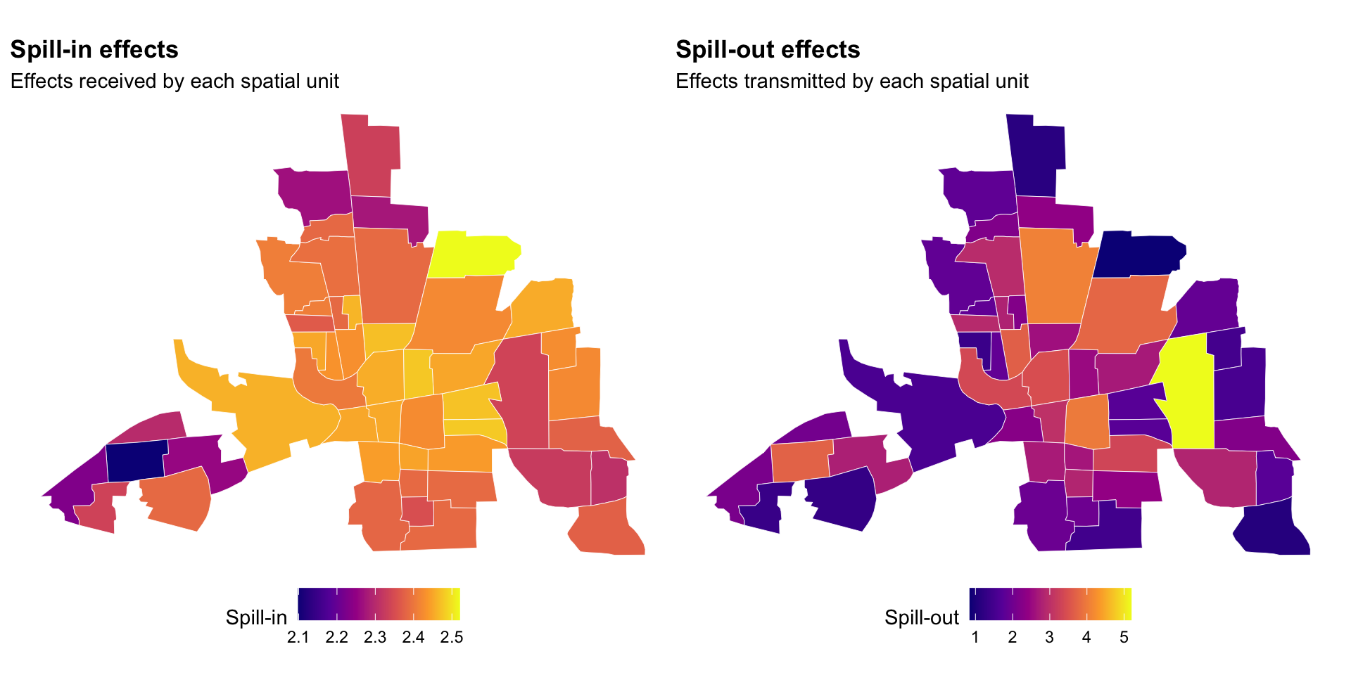
5.9.7 Propagation from One Origin through Successive Rounds
The final impact matrix describes the equilibrium comparative static. To show how that impact is assembled, we use the Neumann expansion discussed in Section 2.4.5: \[ \mathbf S_{\mathrm{policy}} = \widehat\beta_{\mathrm{policy}} \sum_{h=0}^{\infty} \widehat\rho^{h} \mathbf W^{h}. \]
Let \(\mathbf e_j\) denote a vector with one in origin neighborhood \(j\) and zero elsewhere. The effect generated by a one-unit change in policy in that neighborhood during round \(h\) is \[
\mathbf c_j^{(h)}
=
\widehat\beta_{\mathrm{policy}}
\widehat\rho^{h}
\mathbf W^{h}
\mathbf e_j.
\tag{5.31}\]
The cumulative effect through round \(H\) is \[ \mathbf s_j^{(H)} = \sum_{h=0}^{H} \mathbf c_j^{(h)}. \tag{5.32}\]
Column \(j\) is used because the experiment changes the regressor in origin unit \(j\) and records the resulting effects on every destination.
For visual clarity, we choose the neighborhood closest to the geographic center of the study area. This selection has no econometric significance and can be replaced by any neighborhood of substantive interest.
columbus_points <- sf::st_point_on_surface(columbus_map)Warning: st_point_on_surface assumes attributes are constant over geometriescolumbus_center <- sf::st_centroid(sf::st_union(columbus_map))
origin_id <- which.min(as.numeric(sf::st_distance(columbus_points,
columbus_center))
)
origin_polygon <- columbus_map[origin_id, ]
origin_id[1] 25The following function computes each order-specific contribution without forming \(\mathbf W^h\) explicitly. After a round is recorded, multiplication by \(\mathbf W\) advances the effect to the next propagation order.
slm_origin_rounds <- function(W, rho, beta, origin, max_round = 6L) {
  n <- nrow(W)
  if (origin < 1L ||origin > n) {
    stop("origin must identify a row and column of W.", call. = FALSE)
  }

  origin_vector <- numeric(n)
  origin_vector[origin] <- 1

  walk_weights <- origin_vector
  cumulative_effect <- numeric(n)
  results <- vector("list", max_round + 1L)

  for (h in 0:max_round) {
    round_effect <- beta * rho^h * walk_weights
    cumulative_effect <- cumulative_effect + round_effect
    results[[h + 1L]] <- data.frame(unit = seq_len(n),
                                    round = h,
                                    round_effect = as.numeric(round_effect),
                                    cumulative_effect = as.numeric(cumulative_effect))
    walk_weights <- as.numeric(W %*% walk_weights)
  }

  do.call(rbind,results)
}
columbus_origin_rounds <- slm_origin_rounds(W = W_columbus,
rho = columbus_policy_impacts$rho,
beta = columbus_policy_impacts$beta,
origin = origin_id,
max_round = 6L
)Round zero is the initial own-unit effect. Round one distributes the first feedback through \(\mathbf W\), and later rounds contain the effects associated with progressively longer weighted walks. As emphasized in Chapter 2, these are propagation rounds, not mutually exclusive geographic distance bands.
5.9.8 How Much Does Each Round Contribute?
Before mapping the results, we summarize the total amount generated in each round and the cumulative amount through that round.
columbus_round_summary <- aggregate(
  cbind(round_effect, cumulative_effect) ~ round,
  data = columbus_origin_rounds,
  FUN = sum
)

names(columbus_round_summary) <- c(
  "round",
  "total_generated_in_round",
  "total_generated_through_round"
)

full_origin_effect <-
  columbus_policy_impacts$impact_matrix[, origin_id]

full_total_from_origin <- sum(
  full_origin_effect
)

columbus_round_summary$share_of_full_total <-
  columbus_round_summary$total_generated_through_round /
  full_total_from_origin

columbus_round_summary
round total_generated_in_round total_generated_through_round
1 0 0.8867741 0.8867741
2 1 0.7811839 1.6679581
3 2 0.6813822 2.3493403
4 3 0.5062080 2.8555483
5 4 0.4005764 3.2561246
6 5 0.3021103 3.5582350
7 6 0.2317679 3.7900028
share_of_full_total
1 0.1972241
2 0.3709643
3 0.5225079
4 0.6350918
5 0.7241824
6 0.7913737
7 0.8429203Because the weights are row standardized rather than column standardized, the sum of a particular column of \(\mathbf W^h\) need not equal one. Therefore, the amount transmitted from this particular origin can vary with its position in the network.
5.9.9 Preparing the Round-by-Round Maps
We now report magnitudes in the table above and use two normalized map measures for visualization:
- within-round intensity, which divides each round-specific effect by the largest effect in that round;
- fraction of the exact effect accumulated, which compares the cumulative effect through round \(H\) with the exact equilibrium effect for each destination.
The normalization changes only the color display. All impacts and summaries continue to use the unscaled effects.
columbus_round_maps <- do.call(
  rbind,
  lapply(
    split(
      columbus_origin_rounds,
      columbus_origin_rounds$round
    ),
    function(round_data) {
      map_data <- columbus_map
      map_data$round <- round_data$round[1]
      map_data$round_effect <- round_data$round_effect
      map_data$cumulative_effect <- round_data$cumulative_effect

      round_max <- max(
        abs(round_data$round_effect)
      )

      map_data$relative_round_intensity <-
        if (round_max > 0) {
          abs(round_data$round_effect) / round_max
        } else {
          0
        }

      exact_denominator <- pmax(
        abs(full_origin_effect),
        sqrt(.Machine$double.eps)
      )

      map_data$cumulative_share <- pmin(
        abs(round_data$cumulative_effect) / exact_denominator,
        1
      )

      map_data
    }
  )
)

columbus_round_maps$round_label <- factor(
  columbus_round_maps$round,
  levels = 0:6,
  labels = paste("Round", 0:6)
)

columbus_round_maps$cumulative_label <- factor(
  columbus_round_maps$round,
  levels = 0:6,
  labels = paste("Through round", 0:6)
)
5.9.10 Mapping the Spatial Reach of Each Round
The first figure emphasizes where each round travels. Within each panel, a value of one identifies the neighborhood receiving the largest contribution in that round, while zero identifies no contribution. The figure should therefore be read jointly with columbus_round_summary, which retains the absolute magnitude of every round.
plot_columbus_round_effects <-
  ggplot2::ggplot(columbus_round_maps) +
  ggplot2::geom_sf(
    ggplot2::aes(fill = relative_round_intensity),
    color = "white",
    linewidth = 0.20
  ) +
  ggplot2::geom_sf(
    data = origin_polygon,
    fill = NA,
    color = "black",
    linewidth = 0.70,
    inherit.aes = FALSE
  ) +
  ggplot2::facet_wrap(
    ~ round_label,
    ncol = 4
  ) +
  ggplot2::scale_fill_viridis_c(
    name = "Relative intensity",
    limits = c(0, 1),
    option = "C"
  ) +
  ggplot2::coord_sf(datum = NA) +
  ggplot2::labs(
    title = "Spatial reach of successive propagation rounds",
    subtitle = paste(
      "Origin neighborhood:",
      origin_id,
      "— each panel has its own magnitude normalization"
    )
  ) +
  ggplot2::theme_void() +
  ggplot2::theme(
    legend.position = "bottom",
    strip.text = ggplot2::element_text(face = "bold")
  )

plot_columbus_round_effects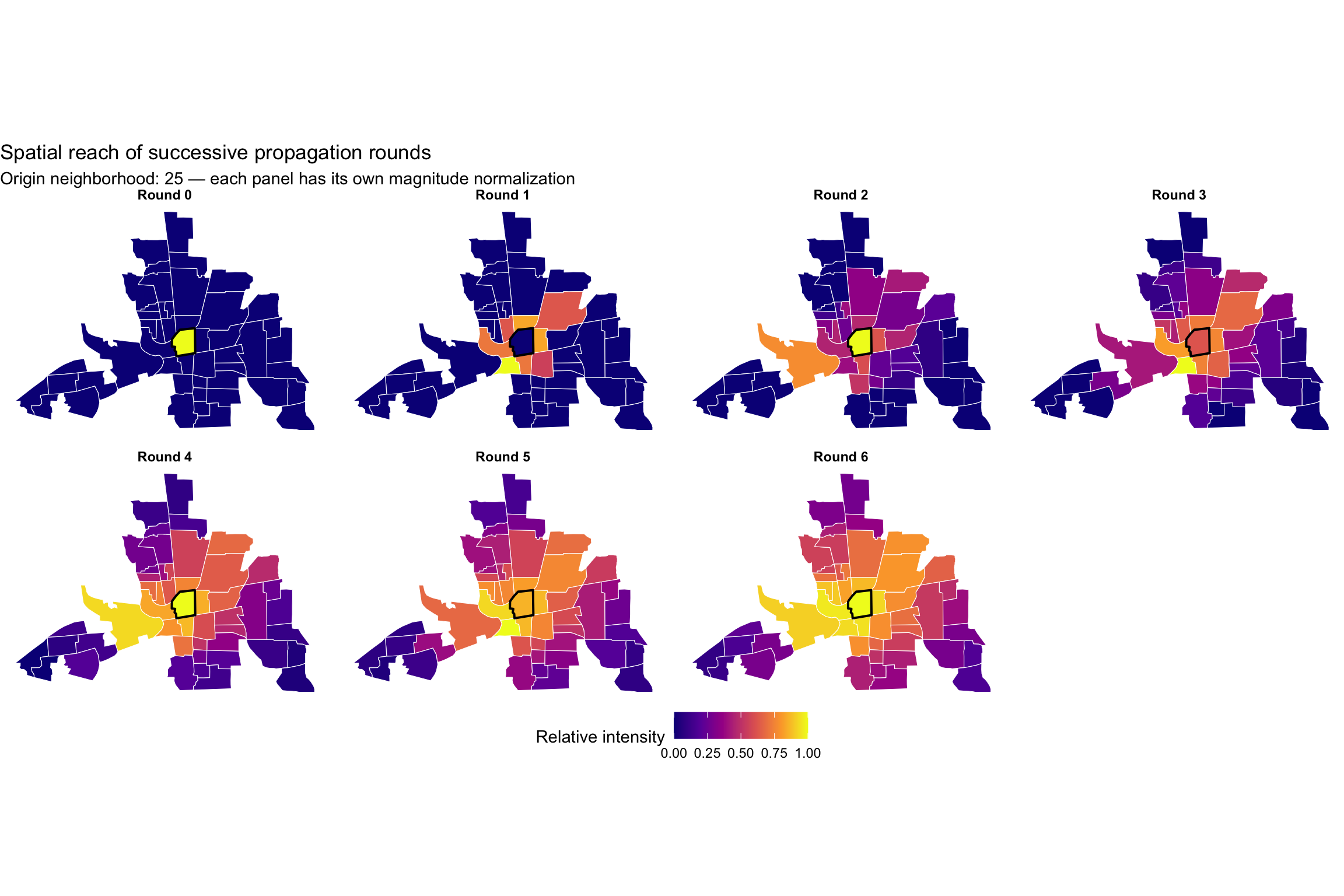
Round zero is concentrated entirely in the origin. Round one reaches its immediate neighbors. Later powers of \(\mathbf W\) spread the effect through progressively longer weighted walks and may revisit neighborhoods reached in earlier rounds.
5.9.11 Mapping Convergence toward the Exact Effect
The second figure asks a different question: how much of the exact equilibrium effect at each destination has been accumulated by round \(H\)? Its fill variable is \[ q_{ij}^{(H)} = \frac{ \left|s_{ij}^{(H)}\right| }{ \left|S_{ij}\right| }, \]
truncated at one only to protect the display against negligible numerical overshooting. Because \(\widehat\beta_{\mathrm{policy}}>0\), \(\widehat\rho>0\), and \(\mathbf W\) is nonnegative, every term in the Neumann expansion is nonnegative. The cumulative effects therefore approach the exact effects monotonically from below.
plot_columbus_cumulative_effects <-
  ggplot2::ggplot(columbus_round_maps) +
  ggplot2::geom_sf(
    ggplot2::aes(fill = cumulative_share),
    color = "white",
    linewidth = 0.20
  ) +
  ggplot2::geom_sf(
    data = origin_polygon,
    fill = NA,
    color = "black",
    linewidth = 0.70,
    inherit.aes = FALSE
  ) +
  ggplot2::facet_wrap(
    ~ cumulative_label,
    ncol = 4
  ) +
  ggplot2::scale_fill_viridis_c(
    name = "Share accumulated",
    limits = c(0, 1),
    option = "C"
  ) +
  ggplot2::coord_sf(datum = NA) +
  ggplot2::labs(
    title = "Convergence of the truncated spatial multiplier",
    subtitle = paste(
      "Effects originating in neighborhood",
      origin_id
    )
  ) +
  ggplot2::theme_void() +
  ggplot2::theme(
    legend.position = "bottom",
    strip.text = ggplot2::element_text(face = "bold")
  )

plot_columbus_cumulative_effects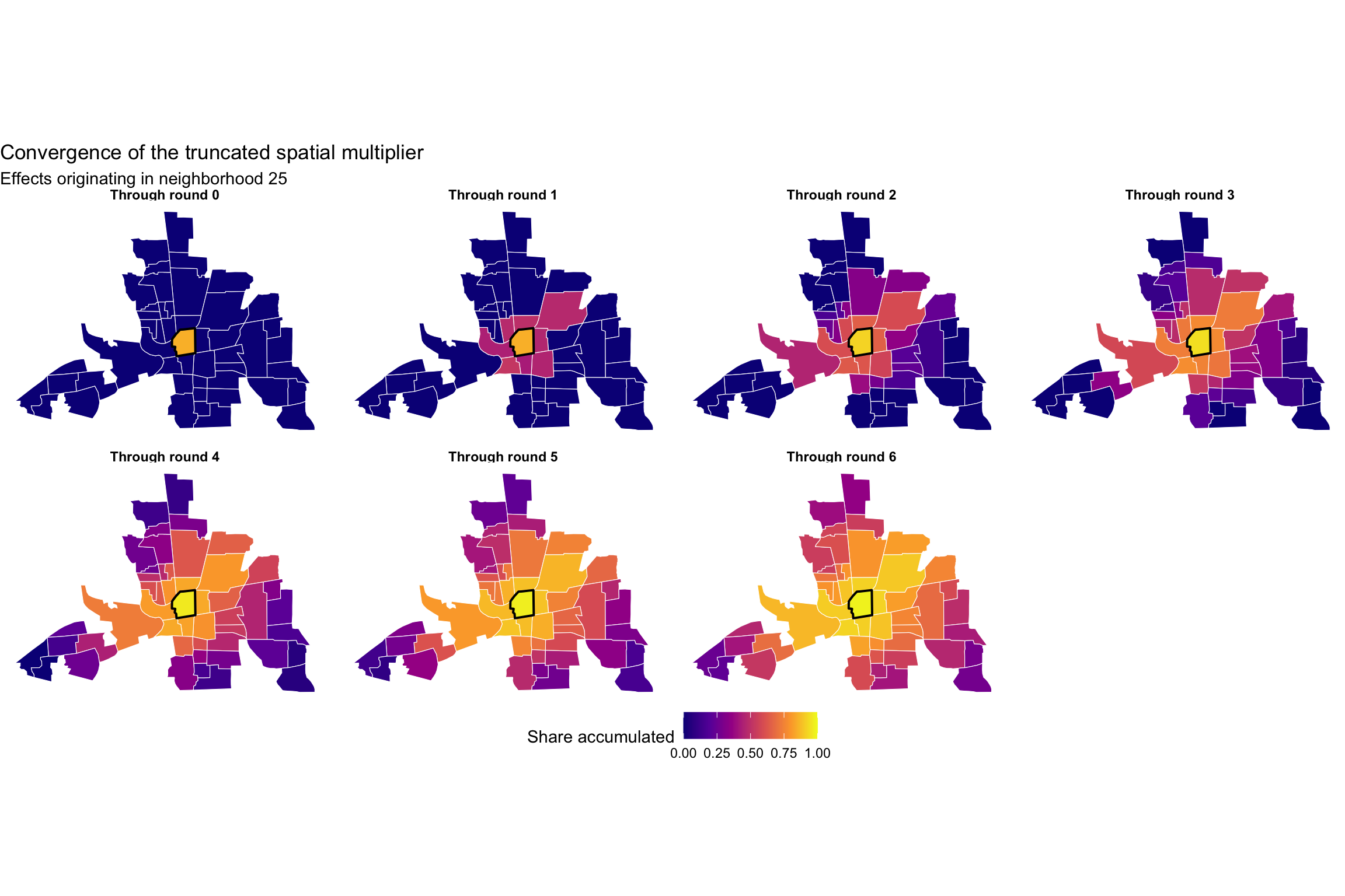
The normalized cumulative map reveals convergence that a raw common scale can hide. It does not imply that all destinations receive effects of the same magnitude; it shows the fraction of each destination’s own exact effect that has been assembled by a given round.
5.9.12 Comparing Round Six with the Exact Multiplier
cumulative_round_6 <- subset(
  columbus_origin_rounds,
  round == 6L
)$cumulative_effect

round_6_remainder <-
  full_origin_effect -
  cumulative_round_6

columbus_round_truncation <- data.frame(
  diagnostic = c(
    "Maximum absolute remainder after round 6",
    "Total effect from exact multiplier",
    "Total effect through round 6",
    "Share of total effect captured through round 6"
  ),
  value = c(
    max(abs(round_6_remainder)),
    full_total_from_origin,
    sum(cumulative_round_6),
    sum(cumulative_round_6) /
      full_total_from_origin
  ),
  row.names = NULL
)

columbus_round_truncation
diagnostic value
1 Maximum absolute remainder after round 6 0.01981052
2 Total effect from exact multiplier 4.49627672
3 Total effect through round 6 3.79000284
4 Share of total effect captured through round 6 0.84292028The truncated expansion is used only for interpretation and visualization. The direct, indirect, total, spill-in, and spill-out effects reported above are calculated from the exact multiplier
\[ \left( \mathbf I_n-\widehat\rho\mathbf W \right)^{-1}, \]
not from the six-round approximation.
5.9.13 Lessons from the Columbus Simulation
This example connects three levels of interpretation.
First, the scalar measures summarize the complete impact matrix:
\[ \widehat{\operatorname{ADI}}, \qquad \widehat{\operatorname{AII}}, \qquad \widehat{\operatorname{ATI}}. \]
Second, the regional measures preserve direction. Spill-in records effects received by a destination, whereas spill-out records effects generated by an origin. They can differ sharply for individual units even though their sample averages are equal.
Third, the Neumann decomposition reveals how one column of the impact matrix is assembled through feedback rounds. Round zero is local, while later rounds propagate through weighted walks and gradually approach the exact equilibrium comparative static.
Finally, the impact standard errors use the QML covariance developed in Chapter 4. The nonlinear transformation from \((\widehat\beta_{\mathrm{policy}},\widehat\rho)\) to the reported impacts retains their estimated covariance and does not treat the spatial parameter as known.
5.10 What We Have Learned
This chapter has implemented the same Gaussian SLM criterion through three numerical routes.
The full maxLik implementation showed how to connect the likelihood, score, and Hessian derived in Chapter 4 to a likelihood-oriented optimizer. The concentrated implementation used the profile formulas from Section 4.3.3 to reduce the search to the scalar parameter \(\rho\). The optim() implementation separated the objective and gradient and used a small cache to avoid repeating identical calculations.
The comparison among these implementations established an important principle: changing the numerical route should not change the estimator when the same criterion and parameter space are used.
The chapter also distinguished alternative covariance estimators for the SLM. Under correct Gaussian specification, inference can be based on either the inverse observed information or the inverse expected information. These estimators are asymptotically equivalent under the maintained Gaussian model, although they need not be numerically identical in finite samples.
Under non-Gaussian but i.i.d. homoskedastic innovations, the point estimator remains the Gaussian QMLE, but inference uses the sandwich covariance from Section 4.6.3.5 and Section 4.6.4. The correction depends on the fitted third and fourth innovation moments and should not be confused with a generic heteroskedasticity or spatial-dependence correction.
Finally, spatialreg was used only after our own implementations were complete. With method = "eigen", its role is to verify the point estimates, the expected-information standard errors, and the maximized likelihood under aligned model, spatial-weights, and Jacobian conventions.
5.11 Exercises
The exercises below extend the programming strategies developed in this chapter. The first asks you to transfer the maximum-likelihood workflow from the SLM to the Spatial Error Model. The second is a guided Monte Carlo exercise based on Lee (2004) and connects computation with the asymptotic arguments developed in Chapter 4.
Exercise 5.1 (Programming the Gaussian MLE for the Spatial Error Model) Consider the Spatial Error Model (SEM) \[ \begin{aligned} \mathbf y &= \mathbf X\boldsymbol\beta+\mathbf u, \\ \mathbf u &= \lambda\mathbf W\mathbf u+\boldsymbol\varepsilon, \\ \boldsymbol\varepsilon &\sim N(\mathbf 0,\sigma^2\mathbf I_n). \end{aligned} \]
The Gaussian likelihood, concentrated likelihood, and Fisher information for this model were derived in Section 4.4.2, Section 4.4.3, and Section 4.4.4.
Your task is to program the Gaussian MLE for the SEM without using a spatial econometrics estimation function. This exercise is about Gaussian maximum likelihood, not Gaussian QML. Do not implement a non-Gaussian sandwich correction.
Add simple coef(), vcov(), logLik(), and summary() methods for your fitted SEM object.
Only after your estimator is complete, estimate the same model using
spatialreg::errorsarlm(
  formula,
  data = data,
  listw = listw_object,
  method = "eigen"
)
Use exactly the same data, spatial weights, and parameterization in the two implementations.
Compare
- \(\widehat{\boldsymbol\beta}\);
- \(\widehat\lambda\);
- \(\widehat\sigma^2\);
- the maximized log-likelihood; and
- the Gaussian information-based standard errors.
Report the numerical differences between your implementation and spatialreg. If the differences are larger than numerical tolerance, identify which component of the implementation is responsible.
Exercise 5.2 (Reproducing the Monte Carlo Design of Lee (2004)) Lee (2004) studies the finite-sample behavior of the Gaussian QMLE under a spatial design in which the number of neighbors may increase with the sample size. This exercise reproduces the Monte Carlo design in Section 7 of that paper.
The exercise is deliberately guided. The main objective is not only to reproduce the reported simulation patterns, but also to understand how the structure of \(\mathbf W_n\) and the regressors affects identification and the rate of convergence of the spatial autoregressive parameter.
- District structure: Suppose there are \(R\) districts and \(m\) units in each district, so that \(n=Rm\). Within each district, every unit assigns equal weight to every other unit. Define \[ \mathbf B_m = \frac{1}{m-1} \left( \mathbf 1_m\mathbf 1_m^\top-\mathbf I_m \right), \] and \[ \mathbf W_n = \mathbf I_R\otimes\mathbf B_m. \]
Verify that every row of \(\mathbf W_n\) sums to one and that there are no links between different districts.
For a vector \(\mathbf a_r=(a_{1r},\ldots,a_{mr})^\top\) belonging to district \(r\), show that \[ \left( \mathbf B_m\mathbf a_r \right)_i = \frac{ \displaystyle\sum_{j=1}^{m}a_{jr}-a_{ir} }{ m-1 }. \]
Use this identity to write a function that computes \(\mathbf W_n\mathbf a\) without constructing the full \(n\times n\) matrix \(\mathbf W_n\). Computational hint: For the largest design, \(R=120\) and \(m=100\), so \(n=12{,}000\). Constructing a dense \(12{,}000\times12{,}000\) matrix in every Monte Carlo replication is unnecessary. Exploit the block structure of the design instead.
- Three data-generating processes: Use \(\lambda_0=0.5\), \(\sigma_0^2=1\). Consider the following three models.
SAR \[ \mathbf y_n = \lambda_0\mathbf W_n\mathbf y_n + \mathbf v_n, \qquad \mathbf v_n\sim N(\mathbf0,\mathbf I_n). \]
MRSAR-1 \[ \mathbf y_n = \lambda_0\mathbf W_n\mathbf y_n + \mathbf x_n\beta_0 + \mathbf v_n, \] where \[ \beta_0=1, \qquad x_{ir}\stackrel{iid}{\sim}N(0,1). \]
Do not include an intercept.
MRSAR-2
Use the same spatial regression model and \(\beta_0=1\), but generate \[ x_{ir} = \frac{z_r+z_{ir}}{\sqrt2}, \] where \[ z_r\stackrel{iid}{\sim}N(0,1), \qquad z_{ir}\stackrel{iid}{\sim}N(0,1), \] with all random variables mutually independent.
Explain the difference between MRSAR-1 and MRSAR-2 in terms of the behavior of the district mean of \(x_{ir}\) as \(m\) increases.
- Simulating \(\mathbf y_n\) efficiently: You could generate the dependent variable from \[ \mathbf y_n = \left( \mathbf I_n-\lambda_0\mathbf W_n \right)^{-1} \left( \mathbf X_n\boldsymbol\beta_0+\mathbf v_n \right), \] but the special block structure makes a full matrix inverse unnecessary. Let \[ \mathbf q_r = \mathbf X_r\boldsymbol\beta_0+\mathbf v_r \] for district \(r\), and let \[ \bar q_r = \frac{1}{m}\mathbf1_m^\top\mathbf q_r. \]
Use the eigenstructure of \(\mathbf B_m\) to verify that \[ \mathbf y_r = \frac{\bar q_r}{1-\lambda_0}\mathbf1_m + \frac{ \mathbf q_r-\bar q_r\mathbf1_m }{ 1+\lambda_0/(m-1) }. \]
Program the simulation using this formula rather than repeatedly solving a large linear system.
- An efficient log-determinant: Show that \(\mathbf B_m\) has eigenvalue \(1\) once and eigenvalue \(-\frac{1}{m-1}\) with multiplicity \(m-1\). Hence show that \[ \log \left| \det \left( \mathbf I_n-\lambda\mathbf W_n \right) \right| = R \left[ \log(1-\lambda) + (m-1) \log \left( 1+\frac{\lambda}{m-1} \right) \right] \] for \(\lambda\) in the connected admissible interval containing zero.
Use this expression in the Monte Carlo estimator instead of computing an \(n\times n\) determinant.
- Concentrated Gaussian QMLE
For each candidate value of \(\lambda\), compute \[ \mathbf y_n(\lambda) = \mathbf y_n-\lambda\mathbf W_n\mathbf y_n. \]
For MRSAR-1 and MRSAR-2, calculate \[ \widehat\beta(\lambda) = \left( \mathbf x_n^\top\mathbf x_n \right)^{-1} \mathbf x_n^\top \mathbf y_n(\lambda). \]
For the pure SAR process there is no regression coefficient to estimate.
Define the fitted innovation vector and compute \[ \widehat\sigma^2(\lambda) = \frac{1}{n} \widehat{\mathbf v}(\lambda)^\top \widehat{\mathbf v}(\lambda). \]
Then maximize \[
\ell_c(\lambda)
=
-\frac{n}{2}
\left[
\log(2\pi)+1+
\log\widehat\sigma^2(\lambda)
\right]
+
\log
\left|
\det
\left(
\mathbf I_n-\lambda\mathbf W_n
\right)
\right|
\] using optimize().
Your estimator should return \[ \widehat\lambda, \qquad \widehat\beta \quad\text{when applicable}, \qquad \widehat\sigma. \]
Notice that the Monte Carlo design uses Gaussian innovations. Therefore, for this particular experiment, the Gaussian QMLE is also the Gaussian MLE. The purpose of the exercise is to study the consequences of the spatial design, not robustness to non-Gaussian innovations.
- Monte Carlo design: Reproduce the design in Lee (2004) using \(R\in\{30,60,120\}\), and \(m\in\{3,5,10,20,50,100\}.\) For every \((R,m)\) combination and each of the three DGPs, use \(B=400\) Monte Carlo replications.
Generate the regressors again in every replication. For each design point, report the empirical mean and empirical standard deviation of \[ \widehat\lambda, \qquad \widehat\beta \quad\text{when applicable}, \qquad \widehat\sigma. \]
Organize the results in tables with \(m\) across columns and \(R\) across blocks, following the structure of Tables I and II in Lee (2004).
Do not expect exact equality with the published Monte Carlo numbers. Different random-number generators and numerical tolerances will generate small differences. The important question is whether you reproduce the qualitative patterns.
- Interpreting the simulation: Use your simulation results to answer the following questions.
- How does the bias of \(\widehat\lambda\) change as \(m\) increases?
- Holding \(R\) fixed, how does the empirical standard deviation of \(\widehat\lambda\) change with \(m\) in the SAR design?
- Is the corresponding pattern similar in MRSAR-1?
- How does MRSAR-2 differ?
- How do the empirical standard deviations of \(\widehat\beta\) and \(\widehat\sigma\) behave as either \(R\) or \(m\) increases?
Now connect these patterns to the asymptotic theory. In this design, \(n=Rm\), \(h_n\asymp m\), so that \[ \sqrt{\frac{n}{h_n}} \asymp \sqrt R. \]
Explain why increasing \(m\) while holding \(R\) fixed need not substantially increase the information about \(\lambda\) in the SAR and MRSAR-1 designs.
Finally, explain why MRSAR-2 behaves differently. Your answer should use the fact that the district-specific component \(z_r\) remains in the district mean of the regressor as \(m\) increases, whereas the district mean of the i.i.d. regressor in MRSAR-1 converges to zero.
- Optional extension: Repeat a subset of the experiment after replacing the Gaussian innovation with a standardized non-Gaussian innovation having mean zero and variance one. The point estimator continues to maximize the Gaussian criterion, but it is now a genuine Gaussian QMLE rather than an MLE. Compare the empirical dispersion of the estimator with standard errors computed from
- the Gaussian expected-information covariance; and
- the QML sandwich covariance developed in Chapter 4.
Explain which covariance estimator is better aligned with the empirical Monte Carlo dispersion and why.