4 Maximum Likelihood Estimation: Theory

This chapter begins the study of estimation methods for spatial regression models. We focus first on maximum likelihood (ML), one of the earliest and most widely used approaches in spatial econometrics (see Anselin 1988, chap. 6). The method accounts explicitly for the simultaneity generated by a spatially lagged dependent variable and, under a correctly specified probability model, provides a coherent framework for estimation and inference.

The chapter proceeds in three stages. We first explain why Ordinary Least Squares (OLS) is generally unsuitable for the Spatial Lag Model. We then derive the likelihood, score, concentrated likelihood, and Hessian for the Spatial Lag Model and the Spatial Error Model. Finally, we study the consistency and asymptotic distribution of the Gaussian quasi-maximum likelihood estimator (QMLE), drawing on the regular asymptotic framework of Lee (2004).

The principal asymptotic results developed in this chapter concern the regular case in which the information matrix is nonsingular and the estimator has the usual root-\(n\) rate. Lee’s broader theory also allows the spatial weights to become increasingly diffuse and shows that weaker rates may arise when the information about the spatial autoregressive parameter degenerates. We will explain that distinction after establishing the regular case.

4.1 Why OLS Generally Fails in the Spatial Lag Model

Recall from Section 2.1.1 that the Spatial Lag Model contains the spatially lagged dependent variable \(\mathbf W_n\mathbf y_n\) as a regressor. Unlike an ordinary explanatory variable, this spatial lag is jointly determined with \(\mathbf y_n\). It is therefore generally correlated with the innovation vector, even when \(\mathbf W_n\) is fixed and the innovations are mutually independent.

4.1.1 A Zero-Mean Pure Spatial Lag Model

To isolate this simultaneity problem, consider the pure Spatial Lag Model without an intercept or additional explanatory variables: \[ \mathbf y_n = \rho_0\mathbf W_n\mathbf y_n + \boldsymbol\varepsilon_n, \tag{4.1}\] where \(\rho_0\) is the true spatial autoregressive parameter, \(\mathbf W_n\) is a nonrandom \(n\times n\) spatial weights matrix, and \(\mathbb E(\boldsymbol\varepsilon_n)=\mathbf{0}\). Define the spatial filter at the true parameter value by \(\mathbf B_{n0}=\mathbf I_n-\rho_0\mathbf W_n\), and assume that \(\mathbf B_{n0}\) is nonsingular. The reduced form is then \[ \mathbf y_n = \mathbf B_{n0}^{-1}\boldsymbol\varepsilon_n. \tag{4.2}\] This is the same reduced-form operation studied in Section 2.2, now written with an \(n\) subscript to make the sequence of spatial systems explicit.

Premultiplying Equation 4.2 by \(\mathbf W_n\) gives \(\mathbf W_n\mathbf y_n=\mathbf G_n\boldsymbol\varepsilon_n\), where \(\mathbf G_n=\mathbf W_n\mathbf B_{n0}^{-1}\). Thus, the regressor \(\mathbf W_n\mathbf y_n\) is itself a linear transformation of the innovation vector.

If OLS is applied to Equation 4.1 without an intercept, the estimator is \[ \widehat\rho_{\mathrm{OLS},n} = \left[ (\mathbf W_n\mathbf y_n)^{\top} (\mathbf W_n\mathbf y_n) \right]^{-1} (\mathbf W_n\mathbf y_n)^{\top}\mathbf y_n. \tag{4.3}\]

Substituting the structural equation \(\mathbf y_n=\rho_0\mathbf W_n\mathbf y_n+\boldsymbol\varepsilon_n\) into Equation 4.3 yields the exact sampling-error decomposition \[ \begin{aligned} \widehat\rho_{\mathrm{OLS},n}-\rho_0 &= \left[ (\mathbf W_n\mathbf y_n)^{\top} (\mathbf W_n\mathbf y_n) \right]^{-1} (\mathbf W_n\mathbf y_n)^{\top} \boldsymbol\varepsilon_n \\ &= \left( \boldsymbol\varepsilon_n^{\top} \mathbf G_n^{\top}\mathbf G_n \boldsymbol\varepsilon_n \right)^{-1} \boldsymbol\varepsilon_n^{\top} \mathbf G_n^{\top} \boldsymbol\varepsilon_n. \end{aligned} \tag{4.4}\]

Equation 4.4 displays the central difficulty. Both the numerator and denominator are quadratic forms in the same innovation vector.

4.1.2 Endogeneity of the Spatial Lag

Suppose that, conditional on \(\mathbf W_n\), the innovations are independent with \(\mathbb E(\varepsilon_{ni})=0\), and \(\mathbb E(\varepsilon_{ni}^2)=\sigma_0^2\). Using the first-moment formula for quadratic forms from Lemma 3.10, we obtain \[ \begin{aligned} \mathbb E\left[ (\mathbf W_n\mathbf y_n)^{\top} \boldsymbol\varepsilon_n\right] &= \mathbb E\left[ \boldsymbol\varepsilon_n^{\top} \mathbf G_n^{\top} \boldsymbol\varepsilon_n\right] \\ &= \sigma_0^2\operatorname{tr}(\mathbf G_n^{\top}) \\ &= \sigma_0^2\operatorname{tr}(\mathbf G_n). \end{aligned} \tag{4.5}\]

At the level of an individual spatial unit, the source of this endogeneity can be seen clearly. Since \(\mathbf W_n\mathbf y_n=\mathbf G_n\boldsymbol\varepsilon_n\), the spatial lag for unit \(i\) can be written as \[ (\mathbf W_n\mathbf y_n)_i = \sum_{j=1}^n g_{n,ij}\varepsilon_{nj} g_{n,ii}\varepsilon_{ni} + \sum_{j\neq i}g_{n,ij}\varepsilon_{nj}. \tag{4.6}\] This decomposition reveals the key issue. Even though unit \(i\) is not its own neighbor in the original spatial weights matrix, the spatial lag appearing in the \(i\)th equation may contain the unit’s own innovation \(\varepsilon_{ni}\) through the coefficient \(g_{n,ii}\). Consequently, \[ \mathbb E\left[ (\mathbf W_n\mathbf y_n)_i\varepsilon_{ni}\right] = \sigma_0^2g_{n,ii}, \tag{4.7}\] which is zero if \(g_{n,ii} = 0\). Why can \(g_{n,ii}\) be nonzero when \(w_{n,ii}=0\)? The answer is spatial feedback. When the Neumann-series condition in Lemma 2.4 holds, \[ \begin{aligned} \mathbf G_n = \mathbf W_n (\mathbf I_n-\rho_0\mathbf W_n)^{-1} = \mathbf W_n + \rho_0\mathbf W_n^2 + \rho_0^2\mathbf W_n^3 + \cdots. \end{aligned} \tag{4.8}\] The first term, \(\mathbf W_n\), has a zero diagonal by construction. Higher-order terms, however, need not. For example, \[ (\mathbf W_n^2)_{ii} = \sum_{j=1}^n w_{n,ij}w_{n,ji}, \] which captures two-step paths that start at unit \(i\), move to another unit \(j\), and return to \(i\) (see Section 1.5). Longer powers of \(\mathbf W_n\) capture analogous longer feedback paths. The economic mechanism is therefore \[ \varepsilon_{ni} \longrightarrow y_{ni} \longrightarrow y_{nj} \longrightarrow (\mathbf W_n\mathbf y_n)_i. \] An innovation affecting unit \(i\) changes its own outcome. Because neighboring units depend on spatially lagged outcomes, this change propagates to their outcomes and can subsequently feed back into the spatial lag of unit \(i\). This feedback mechanism is what makes \(\mathbf W_n\mathbf y_n\) endogenous.

Notice that the feedback channel disappears when \(\rho_0=0\). In that case, \(\mathbf G_n=\mathbf W_n\), so that \(g_{n,ii}=w_{n,ii}=0\) when the spatial weights matrix has a zero diagonal. Thus, the endogeneity described above is not created merely by computing a spatial lag. It arises from the simultaneous spatial feedback generated by the spatial autoregressive model.

4.1.3 Probability Limit of the OLS Estimator

The following proposition applies the quadratic-form Law of Large Numbers from Chapter 3.

Proposition 4.1 (Probability Limit of OLS in the Pure Spatial Lag Model) For each \(n\), suppose that:

\(\boldsymbol\varepsilon_n\) has i.i.d. elements with mean zero, variance \(\sigma_0^2>0\), and finite fourth moment;
\(\mathbf W_n\) is nonrandom and \(\mathbf B_{n0}=\mathbf I_n-\rho_0\mathbf W_n\) is nonsingular;
the absolute row and column sums of \(\mathbf G_n=\mathbf W_n\mathbf B_{n0}^{-1}\) are uniformly bounded;
the limits \[ \tau_G = \lim_{n\to\infty} \frac{1}{n}\operatorname{tr}(\mathbf G_n) \] and \[ q_G = \lim_{n\to\infty} \frac{1}{n} \operatorname{tr} (\mathbf G_n^{\top}\mathbf G_n) >0 \] exist.

Then \[ \widehat\rho_{\mathrm{OLS},n} \overset{p}{\longrightarrow} \rho_0+\frac{\tau_G}{q_G}. \tag{4.9}\] Consequently, OLS is inconsistent whenever \(\tau_G\neq0\).

Proof. Start from the exact decomposition in Equation 4.4 and divide the numerator and denominator by \(n\): \[ \widehat\rho_{\mathrm{OLS},n}-\rho_0 = \frac{ n^{-1}\boldsymbol\varepsilon_n^{\top} \mathbf G_n^{\top} \boldsymbol\varepsilon_n }{ n^{-1}\boldsymbol\varepsilon_n^{\top} \mathbf G_n^{\top}\mathbf G_n \boldsymbol\varepsilon_n }. \tag{4.10}\]

Step 1: Probability limit of the numerator.

Uniform boundedness of the row and column sums of \(\mathbf G_n\) implies the same property for \(\mathbf G_n^{\top}\). Applying Corollary 3.3 with \(\mathbf A_n=\mathbf G_n^{\top}\) gives \[ \begin{aligned} \frac{1}{n} \boldsymbol\varepsilon_n^{\top} \mathbf G_n^{\top} \boldsymbol\varepsilon_n \overset{p}{\longrightarrow} \sigma_0^2 \lim_{n\to\infty} \frac{1}{n} \operatorname{tr}(\mathbf G_n^{\top}) = \sigma_0^2\tau_G. \end{aligned} \tag{4.11}\]

Step 2: Probability limit of the denominator.

By Lemma 3.6, the row and column sums of \(\mathbf G_n^{\top}\mathbf G_n\) are uniformly bounded. Applying Corollary 3.3 again, now with \(\mathbf A_n=\mathbf G_n^{\top}\mathbf G_n\), yields \[ \begin{aligned} \frac{1}{n} \boldsymbol\varepsilon_n^{\top} \mathbf G_n^{\top}\mathbf G_n \boldsymbol\varepsilon_n \overset{p}{\longrightarrow} \sigma_0^2 \lim_{n\to\infty} \frac{1}{n} \operatorname{tr} (\mathbf G_n^{\top}\mathbf G_n) = \sigma_0^2q_G. \end{aligned} \tag{4.12}\] The assumption \(q_G>0\) and the condition \(\sigma_0^2>0\) imply that the limit is strictly positive.

Step 3: Probability limit of the ratio.

Because the denominator in Equation 4.10 converges in probability to the nonzero constant \(\sigma_0^2q_G\), the inversion result in Lemma 3.4 and the product rules in Theorem 3.5 imply \[ \begin{aligned} \widehat\rho_{\mathrm{OLS},n}-\rho_0 \overset{p}{\longrightarrow} \frac{\sigma_0^2\tau_G}{\sigma_0^2q_G} = \frac{\tau_G}{q_G}. \end{aligned} \] Therefore, \[ \widehat\rho_{\mathrm{OLS},n} \overset{p}{\longrightarrow} \rho_0+\frac{\tau_G}{q_G}. \] This proves the result.

The proposition clarifies both the usual result and an important characteristic. OLS is generally inconsistent because spatial feedback makes \(\tau_G\) nonzero. However, inconsistency is not universal. If the sequence of spatial weights is such that \(\frac{1}{n}\operatorname{tr}(\mathbf G_n) \longrightarrow0\), then OLS may be consistent, provided the denominator remains asymptotically nondegenerate. This characteristic is central to the analysis in Lee (2002), where the behavior of OLS depends on how the spatial weights change with the sample size.

For the regular spatial designs most commonly used in cross-sectional applications, OLS should not be relied upon to estimate the coefficient on \(\mathbf W_n\mathbf y_n\). Maximum likelihood and instrumental-variable or GMM methods address the simultaneity explicitly. The latter methods are studied in Chapter 6 and Chapter 7.

4.2 Monte Carlo Illustration of OLS Bias

We now illustrate the finite-sample behavior of OLS using a simple Monte Carlo experiment. The data-generating process is \[ \mathbf y_n = \rho_0\mathbf W_n\mathbf y_n + \boldsymbol\varepsilon_n, \qquad \boldsymbol\varepsilon_n \sim \mathcal N(\mathbf{0},\mathbf I_n), \] with \(\rho_0=0.7\). The spatial weights matrix is based on rook contiguity for a \(15\times15\) regular lattice, so \(n=225\), and is row-standardized.

The design holds \(\mathbf W_n\) fixed across replications. This isolates sampling variation arising from the innovation vector. In each replication, we solve the reduced form and estimate the zero-intercept regression of \(\mathbf y_n\) on \(\mathbf W_n\mathbf y_n\), matching the model in Equation 4.1.

# Fix the Monte Carlo design.
set.seed(123)
replications <- 500L
n_side       <- 15L
n            <- n_side^2
rho_0        <- 0.7
sigma_0      <- 1

# Construct a fixed row-standardized rook-contiguity weights matrix for a
# 15 x 15 lattice. The same spatial structure is used in every replication.
rook_neighbors <- spdep::cell2nb(nrow = n_side, ncol = n_side, type = "rook")
rook_weights   <- spdep::nb2listw(rook_neighbors, style = "W")
W              <- spdep::listw2mat(rook_weights)

# Compute the spatial multiplier once because W and rho_0 are fixed across
# Monte Carlo replications.
spatial_multiplier <- solve(diag(n) - rho_0 * W)

# In each replication, generate the innovations, solve the reduced form, and
# estimate the pure SLM by OLS without an intercept.
rho_hat_ols <- replicate(replications, {
  epsilon <- stats::rnorm(n, mean = 0, sd = sigma_0)
  y       <- drop(spatial_multiplier %*% epsilon)
  Wy      <- drop(W %*% y)
  drop(crossprod(Wy, y) / crossprod(Wy))
})

The following table reports the Monte Carlo mean, bias, standard deviation, and root mean squared error of the OLS estimator.

Table 4.1: Monte Carlo performance of OLS in the pure Spatial Lag Model

True_value	Mean_estimate	Bias	Standard_deviation	RMSE
0.7	1.035	0.335	0.054	0.339

Figure 4.1 shows the empirical sampling distribution. The solid vertical line marks the true value \(\rho_0=0.7\), while the dashed line marks the Monte Carlo mean.

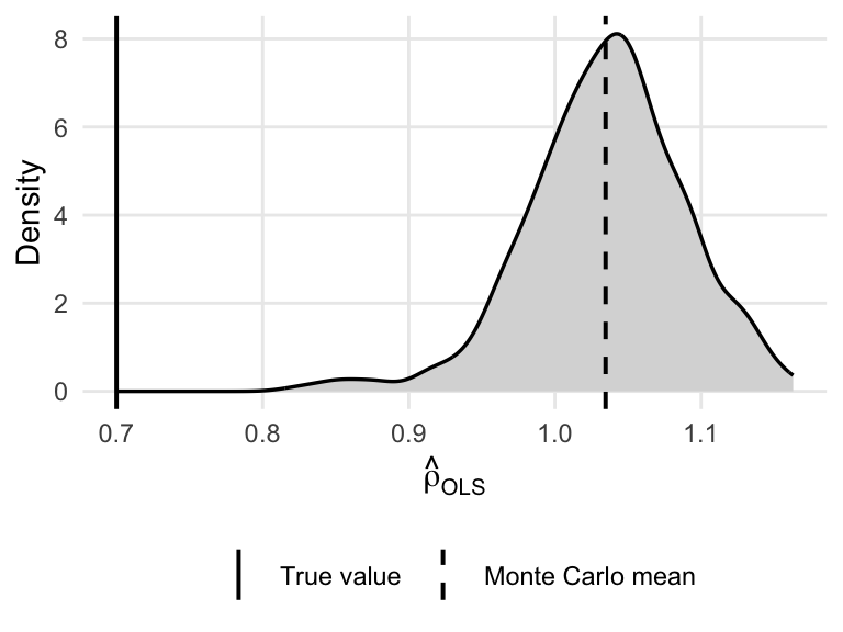
Figure 4.1: Sampling distribution of the OLS estimator in a pure Spatial Lag Model

The simulation shows a substantial upward displacement of the OLS sampling distribution. This direction is consistent with Equation 4.9. In the present design, the spatial weights are nonnegative and \(\rho_0=0.7\). The feedback terms described in Equation 4.8 imply a positive trace contribution, so the asymptotic bias term \(\tau_G/q_G\) is positive. The Monte Carlo distribution is therefore centered above the true value.

Some replications may also produce OLS estimates outside the conventional parameter interval used for the spatial autoregressive coefficient. This is not surprising because OLS estimates \(\rho\) as an unrestricted regression coefficient and does not impose the parameter-space restrictions associated with the spatial model.

An estimate outside this conventional interval does not necessarily imply that \(\mathbf I_n-\widehat\rho_{\mathrm{OLS}}\mathbf W_n\) is singular. Singularity occurs only at particular values satisfying \(\widehat\rho_{\mathrm{OLS}}=\frac{1}{\omega_j}\), for some eigenvalue \(\omega_j\) of \(\mathbf W_n\). Nevertheless, such estimates fall outside the connected parameter region conventionally used to define and estimate the SLM..

4.3 Maximum Likelihood Estimation of the Spatial Lag Model

The simultaneity problem documented in Section 4.1 does not make estimation of the spatial lag model impossible. It does, however, imply that \(\mathbf W_n\mathbf y_n\) cannot be treated as an exogenous regressor in a standard linear regression.

Maximum likelihood approaches the problem differently. Rather than attempting to estimate \(\rho\) from a regression that treats the spatial lag as exogenous, it specifies the joint probability model implied by the simultaneous spatial system. For any candidate value of \(\rho\), the structural equation can be written as \(\mathbf A_n(\rho)\mathbf y_n = \mathbf X_n\boldsymbol\beta + \boldsymbol\varepsilon_n\), where \(\mathbf A_n(\rho) = \mathbf I_n-\rho\mathbf W_n\). Thus, for given parameter values, the model implies the innovations \(\boldsymbol\varepsilon_n = \mathbf A_n(\rho)\mathbf y_n - \mathbf X_n\boldsymbol\beta\). This is the key distinction from OLS. Maximum likelihood does not require \(\mathbf W_n\mathbf y_n\) to be exogenous. Instead, it evaluates how plausible the observed vector \(\mathbf y_n\) is under the entire spatial system implied by each candidate parameter vector.

Under Gaussian innovations, this leads to the Gaussian likelihood of the spatial lag model. The transformation from \(\mathbf y_n\) to \(\boldsymbol\varepsilon_n\) depends on \(\rho\), so its Jacobian must also enter the likelihood. As we will see, this Jacobian produces the log-determinant term \(\log\left|\det\mathbf A_n(\rho)\right|\), which is a defining feature of maximum likelihood estimation in spatial autoregressive models.

4.3.1 The Model and Its Spatial Transformation

Consider the Spatial Lag Model \[ \mathbf y_n = \rho\mathbf W_n\mathbf y_n + \mathbf X_n\boldsymbol\beta + \boldsymbol\varepsilon_n, \tag{4.13}\] where \(\mathbf y_n\) is \(n\times1\), \(\mathbf X_n\) is \(n\times k\), \(\boldsymbol\beta\) is \(k\times1\), and \(\mathbf W_n\) is a known \(n\times n\) spatial weights matrix. For the exact Gaussian likelihood, assume \[ \boldsymbol\varepsilon_n \sim \mathcal N \left( \mathbf 0, \sigma^2\mathbf I_n \right). \tag{4.14}\]

Define \[ \mathbf A_n(\rho) = \mathbf I_n-\rho\mathbf W_n \tag{4.15}\] and the innovation implied by a candidate parameter vector as \[ \boldsymbol\varepsilon_n(\boldsymbol\beta,\rho) = \mathbf A_n(\rho)\mathbf y_n - \mathbf X_n\boldsymbol\beta. \tag{4.16}\]

The parameter vector is \(\boldsymbol\theta=\left(\boldsymbol\beta^{\top},\rho,\sigma^2\right)^{\top}\). The admissible parameter space for \(\rho\) must contain only values for which \(\mathbf A_n(\rho)\) is nonsingular. This is not merely a numerical restriction: without nonsingularity, the structural system does not determine a unique reduced form (see Section 2.2). When \(\mathbf A_n(\rho)\) is nonsingular, \[ \mathbf y_n = \mathbf A_n(\rho)^{-1} \left( \mathbf X_n\boldsymbol\beta + \boldsymbol\varepsilon_n \right). \tag{4.17}\] Consequently, \[ \begin{aligned} \mathbb E \left( \mathbf y_n\right) &= \mathbf A_n(\rho)^{-1} \mathbf X_n\boldsymbol\beta, \\ \operatorname{Var} \left( \mathbf y_n\right) &= \sigma^2 \mathbf A_n(\rho)^{-1} \mathbf A_n(\rho)^{-\top}. \end{aligned} \tag{4.18}\]

Thus, even though the innovations are conditionally independent, the elements of \(\mathbf y_n\) are generally dependent. The likelihood must account for this joint dependence.

4.3.2 Deriving the Joint Density

The observed random vector is \(\mathbf y_n\), whereas the simple Gaussian density in Equation 4.14 is written for \(\boldsymbol\varepsilon_n\). We therefore use the change-of-variables theorem. For fixed \(\mathbf X_n\) and \(\mathbf W_n\), the transformation from \(\mathbf y_n\) to \(\boldsymbol\varepsilon_n\) is \(\boldsymbol\varepsilon_n=\mathbf A_n(\rho)\mathbf y_n-\mathbf X_n\boldsymbol\beta\). Its Jacobian matrix is \[ \frac{ \partial\boldsymbol\varepsilon_n }{ \partial\mathbf y_n^{\top} } = \mathbf A_n(\rho), \tag{4.19}\] where \(\mathbf A_n(\rho)\) is defined in Equation 4.15, so the absolute Jacobian determinant is¹ \[ \left| \det\mathbf A_n(\rho) \right|. \tag{4.20}\]

The density of the innovation vector is \[ f_{\boldsymbol\varepsilon} \left( \boldsymbol\varepsilon_n; \sigma^2 \right) = (2\pi\sigma^2)^{-n/2} \exp \left\{ - \frac{ \boldsymbol\varepsilon_n^{\top} \boldsymbol\varepsilon_n }{2\sigma^2} \right\}. \]

Applying the change-of-variables formula gives \[ \begin{aligned} f_{\mathbf y} \left( \mathbf y_n; \boldsymbol\theta \right) &= (2\pi\sigma^2)^{-n/2} \left| \det\mathbf A_n(\rho) \right| \\ &\quad\times \exp \left\{ - \frac{1}{2\sigma^2} \left[ \mathbf A_n(\rho)\mathbf y_n - \mathbf X_n\boldsymbol\beta \right]^{\top} \left[ \mathbf A_n(\rho)\mathbf y_n - \mathbf X_n\boldsymbol\beta \right] \right\}. \end{aligned} \tag{4.21}\]

Proposition 4.2 (Gaussian log-likelihood for the Spatial Lag Model) Under Equation 4.13 and Equation 4.14, the conditional log-likelihood is \[ \begin{aligned} \ell_n(\boldsymbol\theta) &= - \frac n2\log(2\pi) - \frac n2\log(\sigma^2) + \log \left| \det\mathbf A_n(\rho) \right| \\ &\quad- \frac{1}{2\sigma^2} \boldsymbol\varepsilon_n(\boldsymbol\beta,\rho)^{\top} \boldsymbol\varepsilon_n(\boldsymbol\beta,\rho). \end{aligned} \tag{4.22}\]

The first two terms are the familiar normal-regression terms. The quadratic term measures the fit of the transformed model. The additional log-determinant term adjusts the density for the transformation from \(\boldsymbol\varepsilon_n\) to \(\mathbf y_n\).

The determinant term (i.e., Equation 4.20) is necessary because \(\rho\) enters not only the transformed innovations but also the transformation that maps \(\mathbf y_n\) into \(\boldsymbol\varepsilon_n\). When different candidate values of \(\rho\) are considered, they generate different transformations \(\mathbf A_n(\rho)\). Therefore, their quadratic terms cannot be compared as if all transformations had the same Jacobian. If the log-determinant were omitted, estimation would select \(\rho\) only by making \(\boldsymbol\varepsilon_n(\boldsymbol\beta,\rho)^{\top}\boldsymbol\varepsilon_n(\boldsymbol\beta,\rho)\) small. This would define a nonlinear least-squares criterion, not the Gaussian likelihood of the observed vector \(\mathbf y_n\). The factor \(\left|\det\mathbf A_n(\rho)\right|\) is precisely the adjustment required by the change-of-variables formula derived above.²

4.3.3 Concentrating Out \(\boldsymbol\beta\) and \(\sigma^2\)

Direct maximization of Equation 4.22 is possible, but it is not necessary (see Chapter 5 for a practical perspective). For every admissible value of \(\rho\), the maximizing values of \(\boldsymbol\beta\) and \(\sigma^2\) are available in closed form. Substituting them into the likelihood reduces the numerical optimization to one dimension.

For fixed \(\rho\), differentiate Equation 4.22 with respect to \(\boldsymbol\beta\): \[ \frac{ \partial\ell_n(\boldsymbol\theta) }{ \partial\boldsymbol\beta } = \frac{1}{\sigma^2} \mathbf X_n^{\top} \left[ \mathbf A_n(\rho)\mathbf y_n - \mathbf X_n\boldsymbol\beta \right]. \tag{4.23}\] Setting this expression equal to zero gives \[ \widehat{\boldsymbol\beta}_n(\rho) = \left( \mathbf X_n^{\top}\mathbf X_n \right)^{-1} \mathbf X_n^{\top} \mathbf A_n(\rho)\mathbf y_n. \tag{4.24}\] Thus, conditional on \(\rho\) (that is, knowing \(\rho\)), one could obtain \(\widehat{\boldsymbol\beta}_n(\rho)\) regressing the transformed dependent variable \(\mathbf A_n(\rho)\mathbf y_n\) on the untransformed matrix \(\mathbf X_n\). This point distinguishes the SLM from the SEM considered later.

Differentiating with respect to \(\sigma^2\) yields \[ \frac{ \partial\ell_n(\boldsymbol\theta) }{ \partial\sigma^2 } = - \frac{n}{2\sigma^2} + \frac{ \boldsymbol\varepsilon_n(\boldsymbol\beta,\rho)^{\top} \boldsymbol\varepsilon_n(\boldsymbol\beta,\rho) }{2\sigma^4}. \tag{4.25}\]

After substituting \(\widehat{\boldsymbol\beta}_n(\rho)\) into Equation 4.25 and setting the derivative equal to zero, \[ \widehat\sigma_n^2(\rho) = \frac{1}{n} \widehat{\boldsymbol\varepsilon}_n(\rho)^{\top} \widehat{\boldsymbol\varepsilon}_n(\rho), \tag{4.26}\] where \[ \widehat{\boldsymbol\varepsilon}_n(\rho) = \mathbf A_n(\rho)\mathbf y_n - \mathbf X_n\widehat{\boldsymbol\beta}_n(\rho). \]

Note that the divisor is \(n\), not \(n-k\), because Equation 4.26 is the Gaussian maximum likelihood estimator conditional on \(\rho\) rather than the usual unbiased OLS estimator.

Let \[ \mathbf M_n = \mathbf I_n - \mathbf X_n \left( \mathbf X_n^{\top}\mathbf X_n \right)^{-1} \mathbf X_n^{\top} \tag{4.27}\] be the residual-maker matrix. Then, we can write \[ \widehat{\boldsymbol\varepsilon}_n(\rho) = \mathbf M_n\mathbf A_n(\rho)\mathbf y_n \] and \[ \widehat\sigma_n^2(\rho) = \frac{1}{n} \mathbf y_n^{\top} \mathbf A_n(\rho)^{\top} \mathbf M_n \mathbf A_n(\rho) \mathbf y_n. \tag{4.28}\]

A computationally useful representation follows from two auxiliary regressions. Define \[ \begin{aligned} \widehat{\boldsymbol\beta}_{O,n} &= \left( \mathbf X_n^{\top}\mathbf X_n \right)^{-1} \mathbf X_n^{\top}\mathbf y_n, \\ \widehat{\boldsymbol\beta}_{L,n} &= \left( \mathbf X_n^{\top}\mathbf X_n \right)^{-1} \mathbf X_n^{\top}\mathbf W_n\mathbf y_n. \end{aligned} \tag{4.29}\]

Because \(\mathbf A_n(\rho)\mathbf y_n=\mathbf y_n-\rho\mathbf W_n\mathbf y_n\), \[ \widehat{\boldsymbol\beta}_n(\rho) = \widehat{\boldsymbol\beta}_{O,n} - \rho\widehat{\boldsymbol\beta}_{L,n}. \tag{4.30}\]

Define the corresponding auxiliary residuals \[ \begin{aligned} \mathbf e_{O,n} &= \mathbf y_n - \mathbf X_n\widehat{\boldsymbol\beta}_{O,n}, \\ \mathbf e_{L,n} &= \mathbf W_n\mathbf y_n - \mathbf X_n\widehat{\boldsymbol\beta}_{L,n}. \end{aligned} \tag{4.31}\]

Then \[ \widehat{\boldsymbol\varepsilon}_n(\rho) = \mathbf e_{O,n} - \rho\mathbf e_{L,n}, \tag{4.32}\] and \[ \widehat\sigma_n^2(\rho) = \frac{1}{n} \left( \mathbf e_{O,n}-\rho\mathbf e_{L,n} \right)^{\top} \left( \mathbf e_{O,n}-\rho\mathbf e_{L,n} \right). \tag{4.33}\]

The representation in Equation 4.32 also makes the computational advantage of concentration particularly transparent. The residual sum of squares can be written as \[ \begin{aligned} \widehat{\boldsymbol\varepsilon}_n(\rho)^\top \widehat{\boldsymbol\varepsilon}_n(\rho) &= (\mathbf e_{O,n}-\rho\mathbf e_{L,n})^\top (\mathbf e_{O,n}-\rho\mathbf e_{L,n}) \\ &= \mathbf e_{O,n}^\top\mathbf e_{O,n} - 2\rho,\mathbf e_{O,n}^\top\mathbf e_{L,n} + \rho^2\mathbf e_{L,n}^\top\mathbf e_{L,n}. \end{aligned} \]

Hence, once the two auxiliary regressions have been computed, the three quantities \(\mathbf e_{O,n}^\top\mathbf e_{O,n}\), \(\mathbf e_{O,n}^\top\mathbf e_{L,n}\), \(\mathbf e_{L,n}^\top\mathbf e_{L,n}\) do not depend on \(\rho\). Evaluating the residual sum of squares for a new candidate value of \(\rho\) therefore requires only evaluating a quadratic function, rather than estimating a new regression. This is one reason why concentrating the likelihood reduces the numerical problem to an efficient one-dimensional optimization over \(\rho\).

Substituting the conditional maximizers, Equation 4.30 and Equation 4.33, into Equation 4.22 gives the concentrated log-likelihood \[ \begin{aligned} \ell_{c,n}(\rho) = - \frac n2 \left[ \log(2\pi)+1 \right] - \frac n2 \log \widehat\sigma_n^2(\rho) + \log \left| \det\mathbf A_n(\rho) \right|. \end{aligned} \tag{4.34}\]

The estimate \(\widehat\rho_n\) maximizes Equation 4.34 over the admissible parameter interval. The remaining estimates are then recovered as \[ \widehat{\boldsymbol\beta}_n = \widehat{\boldsymbol\beta}_n(\widehat\rho_n) \qquad\text{and}\qquad \widehat\sigma_n^2 = \widehat\sigma_n^2(\widehat\rho_n). \]

Profile-likelihood algorithm for the SLM

Construct \(\mathbf W_n\mathbf y_n\).
Regress \(\mathbf y_n\) on \(\mathbf X_n\) and retain \(\mathbf e_{O,n}\).
Regress \(\mathbf W_n\mathbf y_n\) on \(\mathbf X_n\) and retain \(\mathbf e_{L,n}\).
For each admissible \(\rho\), evaluate \(\widehat\sigma_n^2(\rho)\) from Equation 4.33 and then evaluate \(\ell_{c,n}(\rho)\).
Numerically maximize the one-dimensional profile criterion.
Recover \(\widehat{\boldsymbol\beta}_n\) and \(\widehat\sigma_n^2\) at \(\widehat\rho_n\).

The two auxiliary regressions are performed only once. During the numerical search, the residual sum of squares is a quadratic function of \(\rho\); the main spatially specific computational task is repeatedly evaluating the log-determinant.

Note that maximizing the concentrated likelihood does not define a different estimator from maximizing the full likelihood over \((\boldsymbol\beta,\rho,\sigma^2)\). Because \(\widehat{\boldsymbol\beta}_n(\rho)\) and \(\widehat\sigma_n^2(\rho)\) are the exact conditional maximizers for each candidate value of \(\rho\), both procedures yield the same maximum likelihood estimates when the numerical optimization is successful. Concentration only reduces the dimension of the numerical search (Anselin and Hudak 1992).

4.3.4 The Score Vector

The score is needed both for numerical optimization and for the asymptotic analysis developed later. The following identities are useful (see Anselin 1988, Appendix 6.A): \[ \frac{\partial\mathbf A_n(\rho)}{\partial\rho} = -\mathbf W_n, \]

\[ \frac{\partial}{\partial\rho} \log \left| \det\mathbf A_n(\rho) \right| = -\operatorname{tr} \left[ \mathbf A_n(\rho)^{-1}\mathbf W_n \right], \tag{4.35}\] and \[ \frac{ \partial\boldsymbol\varepsilon_n(\boldsymbol\beta,\rho) }{ \partial\rho } = -\mathbf W_n\mathbf y_n. \tag{4.36}\]

Because the matrices \(\mathbf A_n(\rho)\) and \(\mathbf W_n\) commute, \(\mathbf A_n(\rho)^{-1}\mathbf W_n = \mathbf W_n\mathbf A_n(\rho)^{-1}\) whenever the inverse exists. Define \[ \mathbf G_n(\rho) = \mathbf W_n\mathbf A_n(\rho)^{-1}. \tag{4.37}\]

With the parameter order \(\boldsymbol\theta=(\boldsymbol\beta^{\top},\rho,\sigma^2)^{\top}\), the score vector is \[ \mathbf s_n(\boldsymbol\theta) = \frac{ \partial\ell_n(\boldsymbol\theta) }{ \partial\boldsymbol\theta } = \begin{pmatrix} \mathbf s_{\beta,n}(\boldsymbol\theta) \\[4pt] s_{\rho,n}(\boldsymbol\theta) \\[4pt] s_{\sigma^2,n}(\boldsymbol\theta) \end{pmatrix}, \] where \[ \mathbf s_{\beta,n}(\boldsymbol\theta) = \frac{1}{\sigma^2} \mathbf X_n^{\top} \boldsymbol\varepsilon_n(\boldsymbol\beta,\rho), \tag{4.38}\]

\[ s_{\rho,n}(\boldsymbol\theta) = - \operatorname{tr}\mathbf G_n(\rho) + \frac{1}{\sigma^2} \boldsymbol\varepsilon_n(\boldsymbol\beta,\rho)^{\top} \mathbf W_n\mathbf y_n, \tag{4.39}\] and \[ s_{\sigma^2,n}(\boldsymbol\theta) = - \frac{n}{2\sigma^2} + \frac{1}{2\sigma^4} \boldsymbol\varepsilon_n(\boldsymbol\beta,\rho)^{\top} \boldsymbol\varepsilon_n(\boldsymbol\beta,\rho). \tag{4.40}\]

To verify Equation 4.39, differentiate the quadratic term: \[ \begin{aligned} \frac{\partial}{\partial\rho} \left[ \boldsymbol\varepsilon_n^{\top} \boldsymbol\varepsilon_n \right] = 2 \boldsymbol\varepsilon_n^{\top} \frac{\partial\boldsymbol\varepsilon_n}{\partial\rho} = -2 \boldsymbol\varepsilon_n^{\top} \mathbf W_n\mathbf y_n. \end{aligned} \]

Multiplication by \(-1/(2\sigma^2)\) therefore produces the positive second term in Equation 4.39.

4.3.4.1 The Score at the True Parameter

Let \[ \boldsymbol\theta_0 = \left( \boldsymbol\beta_0^{\top}, \rho_0, \sigma_0^2 \right)^{\top}, \qquad \mathbf A_{n0} = \mathbf A_n(\rho_0), \qquad \mathbf G_{n0} = \mathbf W_n\mathbf A_{n0}^{-1}. \]

At the true parameter, \(\boldsymbol\varepsilon_n\left(\boldsymbol\beta_0,\rho_0\right)=\boldsymbol\varepsilon_n\). Moreover, the reduced form implies \[ \mathbf W_n\mathbf y_n = \mathbf G_{n0}\mathbf X_n\boldsymbol\beta_0 + \mathbf G_{n0}\boldsymbol\varepsilon_n. \tag{4.41}\]

Substituting Equation 4.41 into Equation 4.39 gives \[ \begin{aligned} s_{\rho,n}(\boldsymbol\theta_0) = \frac{1}{\sigma_0^2} \left( \mathbf G_{n0}\mathbf X_n\boldsymbol\beta_0 \right)^{\top} \boldsymbol\varepsilon_n + \frac{1}{\sigma_0^2} \left[ \boldsymbol\varepsilon_n^{\top} \mathbf G_{n0} \boldsymbol\varepsilon_n - \sigma_0^2 \operatorname{tr}\mathbf G_{n0} \right]. \end{aligned} \tag{4.42}\]

This decomposition is central to the asymptotic theory. The first component is a linear form in the innovations. The second is a centered quadratic form. Their moments are governed by the results in Section 3.9, and their joint limiting distribution is covered by Theorem 3.26 under the corresponding regularity conditions.

The score has conditional mean zero at the true parameter. For example, \[ \mathbb E \left[ \boldsymbol\varepsilon_n^{\top} \mathbf G_{n0} \boldsymbol\varepsilon_n \mid \mathbf X_n,\mathbf W_n \right] = \sigma_0^2 \operatorname{tr}\mathbf G_{n0} \] by Lemma 3.10. Hence the trace term in Equation 4.42 exactly centers the quadratic form. This result also provides a useful connection with the OLS problem discussed in Section 4.1. There, the cross-product between \(\mathbf W_n\mathbf y_n\) and the innovations has a nonzero expectation because of spatial feedback. The same cross-product appears in the likelihood score for \(\rho\), but now the derivative of the log-determinant contributes the trace term that centers the score at the true parameter. Thus, maximum likelihood does not ignore the endogeneity of the spatial lag; it accounts for the simultaneity through the joint probability model, with the log-determinant playing an essential role.

4.3.5 The Hessian Matrix

The Hessian matrix records the curvature of the log-likelihood with respect to the parameter vector. It is defined as \[ \mathbf H_n(\boldsymbol\theta) = \frac{ \partial^2\ell_n(\boldsymbol\theta) }{ \partial\boldsymbol\theta \partial\boldsymbol\theta^{\top} }. \]

At this stage, it is important to distinguish the Hessian from the information matrix. The object derived below is the sample Hessian \(\mathbf H_n(\boldsymbol\theta)\). Its negative, \[ \mathbf J_n(\boldsymbol\theta) = -\mathbf H_n(\boldsymbol\theta), \] is the observed information. By contrast, the expected information is obtained by taking the expectation of the negative Hessian: \[ \mathbf I_n(\boldsymbol\theta) = -\mathbb E\left[ \mathbf H_n(\boldsymbol\theta)\right]. \]

These are distinct objects: the observed information depends on the realized sample, whereas the expected information averages that curvature over the probability model. This distinction will become important when constructing alternative estimators of the covariance matrix (see Chapter 5).

The Hessian is also useful computationally because it describes the local curvature of the objective function and can be used by Newton-type optimization algorithms.

Continue to order the parameters as \((\boldsymbol\beta^{\top},\rho,\sigma^2)^{\top}\). Differentiating the score components gives \[ \frac{ \partial^2\ell_n }{ \partial\boldsymbol\beta \partial\boldsymbol\beta^{\top} } = - \frac{1}{\sigma^2} \mathbf X_n^{\top}\mathbf X_n, \tag{4.43}\]

\[ \frac{ \partial^2\ell_n }{ \partial\boldsymbol\beta \partial\rho } = - \frac{1}{\sigma^2} \mathbf X_n^{\top}\mathbf W_n\mathbf y_n, \tag{4.44}\]

\[ \frac{ \partial^2\ell_n }{ \partial\boldsymbol\beta \partial\sigma^2 } = - \frac{1}{\sigma^4} \mathbf X_n^{\top} \boldsymbol\varepsilon_n(\boldsymbol\beta,\rho), \tag{4.45}\]

\[ \frac{ \partial^2\ell_n }{ \partial\rho^2 } = - \operatorname{tr} \left[ \mathbf G_n(\rho)^2 \right] - \frac{1}{\sigma^2} \mathbf y_n^{\top} \mathbf W_n^{\top}\mathbf W_n \mathbf y_n, \tag{4.46}\]

\[ \frac{ \partial^2\ell_n }{ \partial\rho\partial\sigma^2 } = - \frac{1}{\sigma^4} \boldsymbol\varepsilon_n(\boldsymbol\beta,\rho)^{\top} \mathbf W_n\mathbf y_n, \tag{4.47}\] and \[ \frac{ \partial^2\ell_n }{ \partial(\sigma^2)^2 } = \frac{n}{2\sigma^4} - \frac{1}{\sigma^6} \boldsymbol\varepsilon_n(\boldsymbol\beta,\rho)^{\top} \boldsymbol\varepsilon_n(\boldsymbol\beta,\rho). \tag{4.48}\]

For completeness, the derivative of the trace term in Equation 4.46 is \[ \begin{aligned} \frac{\partial}{\partial\rho} \operatorname{tr}\mathbf G_n(\rho) &= \operatorname{tr} \left[ \frac{\partial\mathbf A_n(\rho)^{-1}}{\partial\rho} \mathbf W_n \right] \\ &= \operatorname{tr} \left[ \mathbf A_n(\rho)^{-1} \mathbf W_n \mathbf A_n(\rho)^{-1} \mathbf W_n \right] \\ &= \operatorname{tr} \left[ \mathbf G_n(\rho)^2 \right]. \end{aligned} \]

The full Hessian is therefore \[ \mathbf H_n(\boldsymbol\theta) = \begin{pmatrix} - \dfrac{\mathbf X_n^{\top}\mathbf X_n}{\sigma^2} & - \dfrac{\mathbf X_n^{\top}\mathbf W_n\mathbf y_n}{\sigma^2} & - \dfrac{\mathbf X_n^{\top}\boldsymbol\varepsilon_n}{\sigma^4} \\[12pt] - \dfrac{\mathbf y_n^{\top}\mathbf W_n^{\top}\mathbf X_n}{\sigma^2} & - \operatorname{tr}\left[\mathbf G_n(\rho)^2\right] - \dfrac{\mathbf y_n^{\top}\mathbf W_n^{\top}\mathbf W_n\mathbf y_n}{\sigma^2} & - \dfrac{\boldsymbol\varepsilon_n^{\top}\mathbf W_n\mathbf y_n}{\sigma^4} \\[12pt] - \dfrac{\boldsymbol\varepsilon_n^{\top}\mathbf X_n}{\sigma^4} & - \dfrac{\boldsymbol\varepsilon_n^{\top}\mathbf W_n\mathbf y_n}{\sigma^4} & \dfrac{n}{2\sigma^4} - \dfrac{\boldsymbol\varepsilon_n^{\top}\boldsymbol\varepsilon_n}{\sigma^6} \end{pmatrix}, \tag{4.49}\] where \(\boldsymbol\varepsilon_n=\boldsymbol\varepsilon_n(\boldsymbol\beta,\rho)\) in this display.

Equation 4.49 is therefore the Hessian of the sample log-likelihood, not the expected information matrix. Later, the Hessian and the information matrices will provide distinct routes for constructing covariance estimators. In particular, the negative sample Hessian can be evaluated at the maximum likelihood estimates to obtain the observed information, while the expected information can be evaluated at estimated parameter values to obtain a plug-in information-based covariance estimator. Keeping these objects separate here will make their theoretical and computational roles clearer in Chapter 5.

4.3.6 Computing the Spatial Log-Determinant

The term \(\log\left|\det\left(\mathbf I_n-\rho\mathbf W_n\right)\right|\) must be evaluated repeatedly during optimization. Directly recomputing a dense \(n\times n\) determinant at every candidate value of \(\rho\) can be expensive.

Let \(\omega_{n1},\ldots,\omega_{nn}\) denote the eigenvalues of \(\mathbf W_n\). The determinant identity used by Ord (1975) is \[ \det \left( \mathbf I_n-\rho\mathbf W_n \right) = \prod_{i=1}^{n} \left( 1-\rho\omega_{ni} \right). \tag{4.50}\] This expression also makes the singularities of the spatial transformation immediately visible. For real \(\rho\), the matrix \(\mathbf I_n-\rho\mathbf W_n\) is singular whenever \(1-\rho\omega_{ni}=0\) for a nonzero real eigenvalue, that is, at \[ \rho=\frac{1}{\omega_{ni}}. \] Thus, the same eigenvalues used to compute the determinant also identify the values of \(\rho\) at which the spatial transformation becomes singular. This is the connection between the log-determinant calculation and the parameter-space discussion in Section 2.2.

When the eigenvalues are real, Equation 4.50 gives \[ \log \left| \det \left( \mathbf I_n-\rho\mathbf W_n \right) \right| = \sum_{i=1}^{n} \log \left| 1-\rho\omega_{ni} \right|. \tag{4.51}\]

This identity is exact; it is not an approximation. Its computational advantage is that the eigenvalues are calculated once and then reused at every evaluation of the profile likelihood. After this one-time eigendecomposition, evaluating the log-determinant at a new candidate value of \(\rho\) requires only the scalar operations in Equation 4.51; no new matrix determinant needs to be computed.

If the spectrum is real and \(\omega_{n,\min}<0<\omega_{n,\max}\), a standard connected admissible interval containing zero is \[ \frac{1}{\omega_{n,\min}} < \rho < \frac{1}{\omega_{n,\max}}. \tag{4.52}\]

In the real-spectrum case, for a nonnegative row-standardized matrix, \(\omega_{n,\max}=1\). The lower endpoint nevertheless depends on the smallest eigenvalue and need not equal \(-1\). Restricting \(\rho\) to a compact subset of the admissible interval keeps the spatial multiplier away from singularity (see Section 2.2).

For a nonsymmetric spatial weights matrix, some eigenvalues may be complex. The product identity remains valid, but the term-by-term real logarithm in Equation 4.51 requires appropriate handling of conjugate pairs. Reliable software therefore uses methods designed for the structure of the weights matrix rather than applying a real logarithm mechanically to complex eigenvalues.

For large sparse systems, alternatives include sparse matrix factorizations, trace approximations, and the characteristic-polynomial approach of Smirnov and Anselin (2001). A broader computational discussion is provided by LeSage and Pace (2010). The important conceptual point is that these methods change how the log-determinant is evaluated, not the likelihood being maximized.

4.4 Maximum Likelihood Estimation of the Spatial Error Model

The Spatial Error Model (SEM) places spatial dependence in the disturbance rather than in the conditional mean (see Section 2.1.3). This changes both the consequences of OLS and the form of the transformation used for maximum likelihood.

4.4.1 Model and Consequences for OLS

Consider \[ \begin{aligned} \mathbf y_n &= \mathbf X_n\boldsymbol\beta + \mathbf u_n, \\ \mathbf u_n &= \lambda\mathbf W_n\mathbf u_n + \boldsymbol\varepsilon_n, \\ \boldsymbol\varepsilon_n &\sim \mathcal N \left( \mathbf 0, \sigma^2\mathbf I_n \right). \end{aligned} \tag{4.53}\]

Define \[ \mathbf B_n(\lambda) = \mathbf I_n-\lambda\mathbf W_n. \tag{4.54}\]

When \(\mathbf B_n(\lambda)\) is nonsingular, we can write \[ \mathbf u_n = \mathbf B_n(\lambda)^{-1} \boldsymbol\varepsilon_n \] and therefore \[ \mathbf y_n = \mathbf X_n\boldsymbol\beta + \mathbf B_n(\lambda)^{-1} \boldsymbol\varepsilon_n. \tag{4.55}\]

Using \(\boldsymbol\varepsilon_n\sim\mathcal N\left(\mathbf 0,\sigma^2\mathbf I_n\right)\), we obtain \[ \mathbb E \left( \mathbf u_n\right) = \mathbf 0 \] and \[ \operatorname{Var} \left( \mathbf u_n\right) = \sigma^2 \mathbf B_n(\lambda)^{-1} \mathbf B_n(\lambda)^{-\top}. \tag{4.56}\]

The covariance matrix is generally full. Spatially connected units can have correlated composite disturbances even though the primitive innovations are independent. Its diagonal elements can also differ, so the composite error \(\mathbf u_n\) may be heteroskedastic even when \(\boldsymbol\varepsilon_n\) is homoskedastic.

Suppose that \(\mathbf X_n\) is nonstochastic or that strict exogeneity holds. The OLS estimator is \[ \widehat{\boldsymbol\beta}_{\mathrm{OLS}} = \boldsymbol\beta + \left( \mathbf X_n^{\top}\mathbf X_n \right)^{-1} \mathbf X_n^{\top}\mathbf u_n. \]

Because \(\mathbb E(\mathbf u_n)=\mathbf 0\), \[ \mathbb E \left( \widehat{\boldsymbol\beta}_{\mathrm{OLS}} \right) = \boldsymbol\beta. \tag{4.57}\] Thus, unlike in the SLM, the problem is not simultaneity between a spatial lag of the dependent variable and the innovation. Under suitable large-sample conditions, OLS can also remain consistent. A formal demonstration of this result is left as an exercise; see Exercise 4.2. However, its covariance matrix is \[ \begin{aligned} \operatorname{Var} \left( \widehat{\boldsymbol\beta}_{\mathrm{OLS}}\right) &= \sigma^2 \left( \mathbf X_n^{\top}\mathbf X_n \right)^{-1} \mathbf X_n^{\top} \mathbf B_n(\lambda)^{-1} \mathbf B_n(\lambda)^{-\top} \mathbf X_n \left( \mathbf X_n^{\top}\mathbf X_n \right)^{-1}. \end{aligned} \tag{4.58}\]

This is not the spherical-error formula \(\sigma^2(\mathbf X_n^{\top}\mathbf X_n)^{-1}\). Consequently:

OLS does not exploit the known covariance structure and is generally inefficient relative to GLS;
conventional homoskedastic OLS standard errors are invalid;
spatial dependence must be incorporated into the covariance estimator or into the estimation method.

The phrase “OLS is unbiased but inefficient” therefore requires the exogeneity condition and refers to the coefficient estimator. It does not imply that the usual OLS standard errors remain valid.

4.4.2 Gaussian Likelihood for the SEM

Let \(\mathbf r_n(\boldsymbol\beta)=\mathbf y_n-\mathbf X_n\boldsymbol\beta\). The primitive innovation implied by the SEM is \[ \boldsymbol\varepsilon_n(\boldsymbol\beta,\lambda) = \mathbf B_n(\lambda) \mathbf r_n(\boldsymbol\beta). \tag{4.59}\]

The Jacobian matrix of the transformation from \(\mathbf y_n\) to \(\boldsymbol\varepsilon_n\) is \[ \frac{ \partial\boldsymbol\varepsilon_n }{ \partial\mathbf y_n^{\top} } = \mathbf B_n(\lambda). \]

Therefore, the conditional joint density is \[ \begin{aligned} f_{\mathbf y} \left( \mathbf y_n; \boldsymbol\beta,\lambda,\sigma^2 \right) &= (2\pi\sigma^2)^{-n/2} \left| \det\mathbf B_n(\lambda) \right| \\ &\quad\times \exp \left\{ - \frac{1}{2\sigma^2} \mathbf r_n(\boldsymbol\beta)^{\top} \mathbf B_n(\lambda)^{\top} \mathbf B_n(\lambda) \mathbf r_n(\boldsymbol\beta) \right\}. \end{aligned} \tag{4.60}\]

The log-likelihood is \[ \begin{aligned} \ell_n^{\mathrm{SEM}} \left( \boldsymbol\beta,\lambda,\sigma^2 \right) &= - \frac n2\log(2\pi) - \frac n2\log(\sigma^2) + \log \left| \det\mathbf B_n(\lambda) \right| \\ &\quad- \frac{1}{2\sigma^2} \mathbf r_n(\boldsymbol\beta)^{\top} \mathbf B_n(\lambda)^{\top} \mathbf B_n(\lambda) \mathbf r_n(\boldsymbol\beta). \end{aligned} \tag{4.61}\]

Define the precision factor \[ \boldsymbol\Omega_n(\lambda) = \mathbf B_n(\lambda)^{\top} \mathbf B_n(\lambda). \tag{4.62}\]

Apart from the factor \(1/\sigma^2\), \(\boldsymbol\Omega_n(\lambda)\) is the inverse of the covariance matrix in Equation 4.56. This explains why the quadratic term in Equation 4.61 has the Generalized Least Squares (GLS) form.

4.4.3 Concentrated Likelihood and GLS Interpretation

For fixed \(\lambda\), differentiate Equation 4.61 with respect to \(\boldsymbol\beta\). The first-order condition is \[ \mathbf X_n^{\top} \boldsymbol\Omega_n(\lambda) \left( \mathbf y_n- \mathbf X_n\boldsymbol\beta \right) = \mathbf 0. \] Hence \[ \widehat{\boldsymbol\beta}_n(\lambda) = \left[ \mathbf X_n^{\top} \boldsymbol\Omega_n(\lambda) \mathbf X_n \right]^{-1} \mathbf X_n^{\top} \boldsymbol\Omega_n(\lambda) \mathbf y_n. \tag{4.63}\]

Because \(\boldsymbol\Omega_n(\lambda)=\mathbf B_n(\lambda)^{\top}\mathbf B_n(\lambda)\), this can also be written as \[ \widehat{\boldsymbol\beta}_n(\lambda) = \left[ \mathbf X_n(\lambda)^{\top} \mathbf X_n(\lambda) \right]^{-1} \mathbf X_n(\lambda)^{\top} \mathbf y_n(\lambda), \tag{4.64}\] where \[ \mathbf y_n(\lambda) = \mathbf B_n(\lambda)\mathbf y_n = \mathbf y_n- \lambda\mathbf W_n\mathbf y_n \] and \[ \mathbf X_n(\lambda) = \mathbf B_n(\lambda)\mathbf X_n = \mathbf X_n- \lambda\mathbf W_n\mathbf X_n. \]

For known \(\lambda\), the Gaussian ML estimator of \(\boldsymbol\beta\) is therefore the GLS estimator and can be computed as OLS using the transformed dependent variable and transformed regressors. This is often called the spatial Cochrane–Orcutt transformation.

The profile estimator of the innovation variance is \[ \widehat\sigma_n^2(\lambda) = \frac{1}{n} \widehat{\boldsymbol\varepsilon}_n(\lambda)^{\top} \widehat{\boldsymbol\varepsilon}_n(\lambda), \tag{4.65}\] where \[ \widehat{\boldsymbol\varepsilon}_n(\lambda) = \mathbf B_n(\lambda) \left[ \mathbf y_n- \mathbf X_n \widehat{\boldsymbol\beta}_n(\lambda) \right]. \]

Substitution into Equation 4.61 gives \[ \begin{aligned} \ell_{c,n}^{\mathrm{SEM}}(\lambda) = - \frac n2 \left[ \log(2\pi)+1 \right] - \frac n2 \log \widehat\sigma_n^2(\lambda) + \log \left| \det\mathbf B_n(\lambda) \right|. \end{aligned} \tag{4.66}\]

The minus sign before \(\frac n2\log\widehat\sigma_n^2(\lambda)\) is essential. A larger transformed residual variance lowers, rather than raises, the concentrated likelihood.

Profile-likelihood algorithm for the SEM

For each admissible candidate value of \(\lambda\):

Form \(\mathbf B_n(\lambda)\).
Transform both the outcome and regressors: \(\mathbf y_n(\lambda)=\mathbf B_n(\lambda)\mathbf y_n\) and \(\mathbf X_n(\lambda)=\mathbf B_n(\lambda)\mathbf X_n\).
Regress \(\mathbf y_n(\lambda)\) on \(\mathbf X_n(\lambda)\) to obtain \(\widehat{\boldsymbol\beta}_n(\lambda)\).
Compute \(\widehat\sigma_n^2(\lambda)\) from the transformed residuals.
Evaluate Equation 4.66.

A one-dimensional optimizer selects \(\widehat\lambda_n\). The estimates \(\widehat{\boldsymbol\beta}_n\) and \(\widehat\sigma_n^2\) are then evaluated at \(\widehat\lambda_n\).

This profile procedure does not require a separate manual alternating algorithm. The numerical optimizer supplies candidate values of \(\lambda\), and the closed-form conditional estimates are recalculated at each evaluation.

As in the SLM, concentrating out \(\boldsymbol\beta\) and \(\sigma^2\) changes only the dimension of the numerical optimization problem; it does not define a different maximum likelihood estimator.

4.4.4 Score and Fisher Information Matrix for the SEM

Define \[ \mathbf G_{B,n}(\lambda) = \mathbf W_n\mathbf B_n(\lambda)^{-1}. \tag{4.67}\]

With parameter order \((\boldsymbol\beta^{\top},\lambda,\sigma^2)^{\top}\), the SEM score is \[ \mathbf s_n^{\mathrm{SEM}} = \begin{pmatrix} \dfrac{1}{\sigma^2} \mathbf X_n^{\top} \mathbf B_n(\lambda)^{\top} \boldsymbol\varepsilon_n \\[10pt] - \operatorname{tr}\mathbf G_{B,n}(\lambda) + \dfrac{1}{\sigma^2} \boldsymbol\varepsilon_n^{\top} \mathbf W_n \mathbf r_n(\boldsymbol\beta) \\[10pt] - \dfrac{n}{2\sigma^2} + \dfrac{1}{2\sigma^4} \boldsymbol\varepsilon_n^{\top} \boldsymbol\varepsilon_n \end{pmatrix}, \tag{4.68}\] where \(\boldsymbol\varepsilon_n=\mathbf B_n(\lambda)\mathbf r_n(\boldsymbol\beta)\).

Let \[ \mathbf H_n^{\mathrm{SEM}}(\boldsymbol\theta) = \frac{ \partial^2\ell_n^{\mathrm{SEM}}(\boldsymbol\theta) }{ \partial\boldsymbol\theta \partial\boldsymbol\theta^{\top} } \] denote the Hessian matrix of the sample log-likelihood. The corresponding expected negative Hessian is \[ \mathcal I_n^{\mathrm{SEM}}(\boldsymbol\theta) = - \mathbb E \left[ \mathbf H_n^{\mathrm{SEM}}(\boldsymbol\theta)\right]. \]

Under correct Gaussian specification, this expected negative Hessian is the Fisher information matrix. For the SEM, \[ \mathcal I_n^{\mathrm{SEM}}(\boldsymbol\theta) = \begin{pmatrix} \dfrac{1}{\sigma^2} \mathbf X_n^{\top} \mathbf B_n(\lambda)^{\top} \mathbf B_n(\lambda) \mathbf X_n & \mathbf 0 & \mathbf 0 \\[12pt] \mathbf 0^{\top} & \operatorname{tr} \left[ \mathbf G_{B,n}(\lambda)^{\top} \mathbf G_{B,n}(\lambda) \right] + \operatorname{tr} \left[ \mathbf G_{B,n}(\lambda)^2 \right] & \dfrac{1}{\sigma^2} \operatorname{tr} \mathbf G_{B,n}(\lambda) \\[12pt] \mathbf 0^{\top} & \dfrac{1}{\sigma^2} \operatorname{tr} \mathbf G_{B,n}(\lambda) & \dfrac{n}{2\sigma^4} \end{pmatrix}. \tag{4.69}\]

Two features are worth emphasizing.

First, the \(\boldsymbol\beta\) block is orthogonal to the covariance parameters under Gaussian normality. This reflects the separation between the conditional mean and covariance structure of the SEM. Second, the \(\lambda\lambda\) element contains \(\operatorname{tr}[\mathbf G_{B,n}(\lambda)^2]\), not the square of \(\operatorname{tr}\mathbf G_{B,n}(\lambda)\). These are different objects: \[ \operatorname{tr} \left[ \mathbf G_{B,n}^2 \right] \neq \left[ \operatorname{tr} \mathbf G_{B,n} \right]^2 \] in general.

Under correct Gaussian specification and regular identification, \[ \widehat{\operatorname{Var}} \left( \widehat{\boldsymbol\theta}_n \right) = \mathcal I_n^{\mathrm{SEM}} \left( \widehat{\boldsymbol\theta}_n \right)^{-1} \] is the information-matrix covariance estimator. As with the SLM, a QMLE based on a misspecified innovation distribution generally requires a sandwich covariance matrix.

4.5 Comparing the SLM and SEM Likelihoods

The two profile-likelihood procedures look similar because both contain a Gaussian fit term and a spatial log-determinant. Their economic and statistical roles are nevertheless different.

Feature	Spatial Lag Model	Spatial Error Model
Location of spatial dependence	Conditional mean of \(\mathbf y_n\) through \(\mathbf A_n(\rho)^{-1}\)	Conditional covariance of \(\mathbf y_n\) through the spatial error process
Structural equation	\(\mathbf A_n(\rho)\mathbf y_n=\mathbf X_n\boldsymbol\beta+\boldsymbol\varepsilon_n\)	\(\mathbf B_n(\lambda)(\mathbf y_n-\mathbf X_n\boldsymbol\beta)=\boldsymbol\varepsilon_n\)
OLS problem	Endogenous spatial lag; generally inconsistent	Generally inefficient; conventional standard errors invalid
Transformation for fixed spatial parameter	Transform \(\mathbf y_n\), not \(\mathbf X_n\)	Transform both \(\mathbf y_n\) and \(\mathbf X_n\)
Profile coefficient estimate	OLS of \(\mathbf A_n(\rho)\mathbf y_n\) on \(\mathbf X_n\)	OLS of \(\mathbf B_n(\lambda)\mathbf y_n\) on \(\mathbf B_n(\lambda)\mathbf X_n\)
Spatial determinant	\(\log\|\det\mathbf A_n(\rho)\|\)	\(\log\|\det\mathbf B_n(\lambda)\|\)

Although the determinant terms have the same algebraic form when the same spatial weights matrix is used, the two likelihoods are not interchangeable. In the SLM, the spatial transformation acts on the dependent variable and changes the conditional mean of the model. In the SEM, it acts on the regression disturbance and changes its covariance structure. The distinction therefore lies not in the appearance of the determinant alone, but in the complete transformation that defines the innovation vector.

In both models, the determinant term is not a penalty added by convention. It is the Jacobian required by the transformation from the observed outcome vector to the primitive innovation vector.

4.6 Asymptotic Properties of the Spatial Lag Model

The previous sections constructed the Gaussian likelihood for the Spatial Lag Model (SLM) and Spatial Error Model (SEM). This section studies the asymptotic properties of the SLM. The analysis follows Lee (2004). The estimator is called a maximum likelihood estimator when the innovations are Gaussian. It is called a Gaussian quasi-maximum likelihood estimator when the same Gaussian criterion is maximized even though the innovation distribution need not be normal.

The distinction matters for inference. Under correct Gaussian specification, the information equality holds and the inverse information matrix is the asymptotic covariance matrix. Under non-Gaussian innovations, the estimator can remain consistent and asymptotically normal, but its covariance matrix generally has the sandwich form.

Scope of the results developed in this section

The main results below cover the regularly identified SLM. In that case, the spatial parameter is identified partly through variation in the conditional mean, and the estimator has the usual root-\(n\) rate. This regular result may hold whether the sequence \(h_n\) introduced below is bounded or divergent. A divergent \(h_n\) does not, by itself, imply a slower rate. The slower rate found by Lee (2004) arises when the mean-based source of identification becomes asymptotically weak and the information about the spatial parameter is supplied mainly by quadratic forms.

4.6.1 Regularity Conditions

As discussed in Section 3.7 spatial asymptotics require a sequence of models indexed by \(n\). We therefore write \(\mathbf y_n = \rho_0\mathbf W_n\mathbf y_n + \mathbf X_n\boldsymbol\beta_0 +\boldsymbol\varepsilon_n\), where the dimension of every object changes with \(n\). Define \[ \mathbf A_n(\rho) = \mathbf I_n-\rho\mathbf W_n, \qquad \mathbf A_{n0} = \mathbf A_n(\rho_0), \] and \[ \mathbf G_{n0} = \mathbf W_n\mathbf A_{n0}^{-1}. \tag{4.70}\]

The following assumptions provide a simpler version of the regular case in Lee (2004). The number of regressors \(k\) is fixed as \(n\) increases.

Assumption 1 (ML1: Innovations)

For every \(n\), the elements of \(\boldsymbol\varepsilon_n\) are independent and identically distributed. Their common distribution does not depend on \(n\) and satisfies \[ \mathbb E(\varepsilon_{ni})=0, \qquad \mathbb E(\varepsilon_{ni}^2)=\sigma_0^2>0. \]

For some \(\gamma>0\), \[ \mathbb E \left( |\varepsilon_{ni}|^{4+\gamma} \right) <\infty. \]

The fourth-moment requirement in Assumption 1 is needed for variances of quadratic forms. The additional positive moment is used by the linear–quadratic central limit theorem. Note that we do not require the normality of the innovations.

Assumption 2 (ML2: Individual spatial weights)

The diagonal of \(\mathbf W_n\) is zero, and its entries satisfy \[ w_{n,ii}=0, \qquad \max_{i,j}|w_{n,ij}| = O\!\left(\frac{1}{h_n}\right), \] where \(h_n\) may be bounded or divergent.

Assumption 2 requires a deeper discussion because it is the first condition that tells us how the spatial weights matrix is allowed to change as the sample grows. This is precisely the issue emphasized in Lee (2004): writing \(n\to\infty\) is not enough in a spatial model unless we also describe the sequence \(\{\mathbf W_n\}\).

The condition \[ \max_{1\leq i,j\leq n} |w_{n,ij}| = O\!\left(\frac{1}{h_n}\right) \] means that there is a finite constant \(C\) such that \[ |w_{n,ij}| \leq \frac{C}{h_n} \] uniformly over \(i\), \(j\), and sufficiently large \(n\). This is the deterministic big-\(O\) notation defined in Definition 3.5, now applied to the triangular-array setting introduced in Section 3.7. The sequence \(h_n\) is therefore a rate sequence for the magnitude of the individual spatial weights. It is not, by definition, the number of neighbors. In many common spatial-weighting schemes, however, the two are closely related.

A useful way to read Assumption 2 is to ask:

If I construct \(\mathbf W_n\) by the same rule for progressively larger samples, what happens to the largest individual weight?

Two broad cases may arise.

If \(h_n\) remains bounded, individual weights are allowed to remain of nonvanishing order. This is the natural case when each unit continues to interact with only a bounded number of relevant neighbors.
If \(h_n\to\infty\), the largest individual weights shrink toward zero. This commonly occurs when the number of relevant neighbors grows with the sample and the weights are spread over an increasingly large neighborhood.

For row-standardized weights, Lee (2004) gives an especially useful interpretation. Suppose the raw nonnegative spatial weights are \(d_{n,ij}\) and \[ w_{n,ij} = \frac{d_{n,ij}} {\sum_{j=1}^{n}d_{n,ij}}. \]

Assume that the raw weights are uniformly bounded, so that for some finite constant \(\bar d\), \(0\leq d_{n,ij}\leq \bar d\), and suppose that the raw row sums are uniformly of order \(h_n\). More precisely, suppose there exist constants \(0<c<C<\infty\) such that, for all sufficiently large \(n\), \[ c h_n \leq \sum_{j=1}^{n}d_{n,ij} \leq C h_n \] uniformly over \(i\). Then \[ 0 \leq w_{n,ij} = \frac{d_{n,ij}} {\sum_{j=1}^{n}d_{n,ij}} \leq \frac{\bar d}{c h_n}. \]

Therefore, \[ \max_{i,j}|w_{n,ij}| = O\left(\frac{1}{h_n}\right), \] which is precisely the scaling required by Assumption 2.

This calculation provides a useful interpretation of \(h_n\): for row-standardized weights, \(h_n\) often measures the order of the total raw neighborhood weight available to each spatial unit before normalization. A particularly simple case occurs when the raw weights are binary. If \[ d_{n,ij} = \begin{cases} 1, & j\in\mathcal N_{n,i},\\ 0, & j\notin\mathcal N_{n,i} \end{cases} \] then \(\sum_{j=1}^{n}d_{n,ij}=|\mathcal N_{n,i}|,\) so \(h_n\) has a direct interpretation as the order of the number of neighbors. This is why, for fixed-\(k\) nearest-neighbor designs or contiguity designs with a uniformly bounded number of neighbors, the natural choice is \(h_n=O(1)\). For more general weights, however, \(h_n\) is a scaling sequence for the weights and should not be identified mechanically with the number of neighbors.

This interpretation clarifies several familiar constructions.

With a fixed-\(k\) nearest-neighbor rule, the number of neighbors does not grow with \(n\). The natural rate is therefore bounded: \(h_n=O(1).\)
With rook or queen contiguity along a sequence of spatial designs for which the number of neighbors remains uniformly bounded, the same conclusion applies: \(h_n=O(1)\). The relevant property is the bounded-neighborhood structure of the sequence, not the label rook or queen by itself.
If unit \(i\) has \(q_n\) approximately equally weighted neighbors and \(q_n\to\infty\), then a typical normalized weight is of order \(1/q_n\), so the natural rate is \(h_n\asymp q_n.\)

The last example also shows why \(h_n\) cannot be inferred mechanically from one observed matrix. Assumption 2 is an asymptotic condition on the rule generating the sequence \(\{\mathbf W_n\}\). The relevant question is how that same construction rule behaves as the spatial sample expands.

Inverse-distance weights without a cutoff provide a useful example in which \(h_n\) can diverge. Consider \(n\) units located at equally spaced points on a line, with distance \(d\) between adjacent units, and define \[ a_{n,ij} = \begin{cases} \dfrac{1}{d_{ij}}, & i\neq j,\\[4pt] 0, & i=j. \end{cases} \]

For an interior unit \(i\), the raw row sum has the approximate form \[ s_{n,i} = \sum_{j\neq i}a_{n,ij} \approx \frac{2}{d} \left( 1+\frac{1}{2}+\frac{1}{3}+\cdots+\frac{1}{m_n} \right), \] where \(m_n\) is the number of distance levels available on either side of the unit. The expression in parentheses is a harmonic sum and is therefore of order \(\log n\). Boundary units have fewer neighbors at some distances, but their raw row sums are still of the same order. Consequently, the row sums of the unnormalized inverse-distance matrix do not remain uniformly bounded as \(n\) grows. This also explains why empirical applications often impose a cutoff distance \(d^*\): on a regular increasing spatial design with fixed spacing, a fixed cutoff can keep the number of relevant neighbors bounded.

Now row-standardize the inverse-distance weights: \[ w_{n,ij} = \frac{a_{n,ij}}{s_{n,i}}. \]

Because \(s_{n,i}\) is of order \(\log n\), the largest normalized weight, assigned to a nearest neighbor, is of order \(1/\log n\). Hence \[ \max_{i,j}|w_{n,ij}| = O\left(\frac{1}{\log n}\right), \] and a natural rate sequence is \(h_n\asymp\log n.\) This example is useful because it shows that row standardization does not force \(h_n\) to be bounded. It can generate a sequence in which every individual weight becomes small as the effective neighborhood expands.

Assumption 3 (ML3: Relative neighborhood growth)

The rate sequence satisfies \[ \frac{h_n}{n} \longrightarrow0. \]

Assumption 3 determines how fast the interaction scale described by \(h_n\) is allowed to grow relative to the sample. If \(h_n\) is bounded, the condition is automatic. Its substantive content appears when \(h_n\to\infty\).

For equal-weight neighborhoods with \(q_n\) neighbors, \(h_n\asymp q_n,\) so Assumption 3 becomes \(\frac{q_n}{n}\longrightarrow0.\) Thus, the number of relevant neighbors may increase with the sample, but its natural scale must grow more slowly than \(n\). For example, if \(q_n=\lfloor n^{1/3}\rfloor,\) then \[ h_n\to\infty, \qquad \frac{h_n}{n} \asymp n^{-2/3} \longrightarrow0. \]

By contrast, a spatial design whose natural neighborhood scale is proportional to the entire sample, \(h_n\asymp n,\) does not satisfy Assumption 3. This is the type of large-neighborhood behavior that Lee (2004) excludes from this regularity condition.

The inverse-distance example above satisfies Assumption 2 with \(h_n\asymp\log n.\) Moreover, \[ \frac{h_n}{n} \asymp \frac{\log n}{n} \longrightarrow0, \] so Assumption 3 is also satisfied.

A second useful example comes directly from the discussion in Lee (2004). Suppose there are \(R_n\) districts and \(m_n\) units in each district, and every unit interacts equally with the other units in its own district. Then \(n=m_nR_n,\) and the natural rate is \(h_n=m_n-1.\) Therefore, \[ \frac{h_n}{n} = \frac{m_n-1}{m_nR_n}. \]

If both the number of units per district and the number of districts increase, with \(R_n\to\infty\), then \[ h_n\to\infty, \qquad \frac{h_n}{n} \longrightarrow0. \]

This example is important because it shows that an increasing number of neighbors does not by itself violate Assumption 3. What matters is the rate at which the neighborhood scale grows relative to the overall sample.

Example 4.1 (Equal-weight neighborhoods) Suppose every unit has \(q_n\) neighbors and the matrix is row-standardized: \[ w_{n,ij} = \begin{cases} 1/q_n, & j\in\mathcal N_{n,i},\\ 0, & j\notin\mathcal N_{n,i}. \end{cases} \]

Then \(h_n=q_n\) is a natural rate sequence. If \(q_n=4\) for every \(n\), then \(h_n\) is bounded. If \(q_n=\lfloor n^{1/3}\rfloor\), then \[ h_n\to\infty, \qquad \frac{h_n}{n} \to0. \]

By contrast, if the natural neighborhood size is a fixed positive fraction of the sample, for example \[ q_n=\lfloor0.25n\rfloor, \] then \[ \frac{h_n}{n} \longrightarrow0.25, \] so Assumption 3 does not hold.

Does my spatial weights matrix satisfy these conditions?

Assumption 2 and Assumption 3 are conditions on a sequence of spatial designs, not mechanical tests for one finite matrix. For an empirical weights matrix, the relevant thought experiment is:

Keep the same rule used to construct the weights.
Apply that rule conceptually to increasingly large spatial samples.
Determine the natural rate governing the largest individual weights or, for row-standardized weights, the natural growth rate of the raw neighborhood weight before normalization.
Identify the corresponding \(h_n\) and check whether \[ \frac{h_n}{n}\to0. \]

Fixed-\(k\) nearest-neighbor matrices and local contiguity matrices with a uniformly bounded neighborhood size typically correspond to \(h_n=O(1)\). When the number of relevant neighbors increases, \(h_n\) may diverge and the relative-growth condition must be checked explicitly. These two conditions are not sufficient by themselves for the later asymptotic arguments. In particular, row standardization does not automatically establish the column-sum and spatial-multiplier requirements in Assumption 5. The concepts needed to assess those requirements were developed in Section 3.8.

Assumption 4 (ML4: Existence of the true reduced form)

The matrix \(\mathbf A_{n0}=\mathbf I_n-\rho_0\mathbf W_n\) is nonsingular for every \(n\).

Assumption 5 (ML5: Uniform control of spatial dependence)

The sequences \(\{\mathbf W_n\}\) and \(\{\mathbf A_{n0}^{-1}\}\) are uniformly bounded in both absolute row and column sums.

The meaning of uniform boundedness in absolute row and column sums and the matrix results used below were developed in Section 3.8; see in particular Definition 3.20. We do not repeat those arguments here. In the present model, Assumption 5 applies those conditions to \(\{\mathbf W_n\}\) and \(\{\mathbf A_{n0}^{-1}\}\) so that spatial interaction and the spatial multiplier remain controlled as \(n\) increases.

Assumption 6 (ML6: Regressors)

The elements of \(\mathbf X_n\) are nonrandom and uniformly bounded. In addition, \[ \frac{1}{n} \mathbf X_n^{\top}\mathbf X_n \longrightarrow \mathbf Q_{xx}, \] where \(\mathbf Q_{xx}\) is finite and positive definite.

This excludes asymptotic multicollinearity among the columns of \(\mathbf X_n\). A stochastic-regressor version is possible, but it requires conditional moment and probability-limit conditions that are not pursued here.

Assumption 7 (ML7: Uniform stability over the parameter space)

The parameter space \(\mathcal R\) for \(\rho\) is compact, \(\rho_0\) lies in its interior, and \(\mathbf A_n(\rho)\) is nonsingular for every \(\rho\in\mathcal R\). Moreover, \(\mathbf A_n(\rho)^{-1}\) is uniformly bounded in either absolute row sums or absolute column sums, uniformly over \(\rho\in\mathcal R\).

This condition keeps the admissible interval away from values at which the spatial multiplier becomes unstable. For a row-standardized nonnegative matrix, a compact subset of \((-1,1)\) is a common sufficient choice. For a matrix with real eigenvalues, the admissible set must remain inside the interval determined by the extreme eigenvalues, as discussed in Section 2.2.

To state the final condition, define the spatially generated regressor \[ \mathbf d_n = \mathbf G_{n0} \mathbf X_n \boldsymbol\beta_0. \tag{4.71}\]

Assumption 8 (ML8: Regular identification)

The limit \[ \frac{1}{n} \begin{pmatrix} \mathbf X_n & \mathbf d_n \end{pmatrix}^{\top} \begin{pmatrix} \mathbf X_n & \mathbf d_n \end{pmatrix} \longrightarrow \mathbf Q_z \tag{4.72}\] exists and \(\mathbf Q_z\) is positive definite.

Assumption 8 is the defining feature of the regular case. It requires the spatially generated regressor \(\mathbf d_n\) to contain asymptotically nonredundant variation after controlling for \(\mathbf X_n\).

4.6.2 Consistency of the Gaussian QMLE

The previous regularity conditions describe the environment in which consistency can be established. We now explain how those assumptions enter the proof. The central idea is the standard extremum-estimator argument, adapted to a triangular array and to the concentrated spatial likelihood.

4.6.2.1 Step 1: Reduce the Problem to the Spatial Parameter

As we established in Section 4.3.3, for every admissible value of \(\rho\), the Gaussian criterion has closed-form maximizers in \(\boldsymbol\beta\) and \(\sigma^2\). Therefore, the estimator can be written as \[ \widehat\rho_n \in \arg\max_{\rho\in\mathcal R} \ell_{c,n}(\rho), \] followed by \[ \widehat{\boldsymbol\beta}_n = \widehat{\boldsymbol\beta}_n(\widehat\rho_n), \qquad \widehat\sigma_n^2 = \widehat\sigma_n^2(\widehat\rho_n). \]

This structure suggests a two-stage proof. We first establish \[ \widehat\rho_n \overset{p}{\longrightarrow} \rho_0. \] Once this result is available, consistency of \(\widehat{\boldsymbol\beta}_n\) and \(\widehat\sigma_n^2\) follows from their profile formulas. Thus, the main task is to understand why the maximizer of the one-dimensional concentrated criterion approaches \(\rho_0\).

Define the normalized sample criterion \[ m_n(\rho) = \frac{1}{n} \ell_{c,n}(\rho) \] and let \[ m_n^0(\rho) = \frac{1}{n} Q_n(\rho) \] be the deterministic population counterpart constructed in Step 4. Two properties are sufficient for consistency of \(\widehat\rho_n\).

First, \(\rho_0\) must be uniquely identified as the maximizer of the population concentrated criterion. For a fixed population criterion, uniqueness means that \[ m^0(\rho) < m^0(\rho_0) \qquad \text{for every }\rho\neq\rho_0. \]

In the present model, however, the criterion forms a triangular array: \(m_n^0(\rho)\) may change with \(n\). Merely requiring \(\rho_0\) to be the unique maximizer of each \(m_n^0(\rho)\) would not be sufficient if the gap between the criterion at \(\rho_0\) and the criterion at incorrect values were allowed to vanish as \(n\) increases. We therefore express uniqueness in the stronger operational form of uniform separation.

For every \(\eta>0\), there must exist \(c_\eta>0\) such that, for all sufficiently large \(n\), \[ \sup_{\substack{ \rho\in\mathcal R\\ |\rho-\rho_0|\geq\eta }} \left[ m_n^0(\rho)-m_n^0(\rho_0) \right] \leq -c_\eta. \tag{4.73}\] This condition says that values of \(\rho\) lying outside any fixed neighborhood of \(\rho_0\) remain uniformly below the population maximum. Thus, uniform separation is not a different identification concept from uniqueness. It is the form of uniqueness required for a triangular-array extremum argument.

Uniqueness and uniform separation

For a fixed continuous population criterion on a compact parameter space, a unique maximizer is strictly separated from all values outside any neighborhood of that maximizer. Here the population criterion is the sequence \(\{m_n^0(\rho)\}\). The additional requirement is that this separating gap does not disappear as \(n\) grows. This is why the uniqueness condition is stated as uniform separation.

Second, the sample criterion must approximate the population criterion uniformly: \[ \sup_{\rho\in\mathcal R} \left| m_n(\rho)-m_n^0(\rho) \right| = o_p(1). \tag{4.74}\]

Uniformity is essential because \(\widehat\rho_n\) is selected after observing the entire random criterion. Convergence at each fixed value of \(\rho\) would not exclude a sample-dependent spurious maximum elsewhere in \(\mathcal R\).

To see how the two properties work together, write \[ \begin{aligned} m_n(\rho)-m_n(\rho_0) = m_n^0(\rho)-m_n^0(\rho_0) + \left[ m_n(\rho)-m_n^0(\rho) \right] - \left[ m_n(\rho_0)-m_n^0(\rho_0) \right]. \end{aligned} \] Away from \(\rho_0\), the uniform-separation form of population uniqueness makes \(m_n^0(\rho)-m_n^0(\rho_0)\) negative by a fixed amount. Uniform convergence makes the two approximation errors jointly smaller than that gap with probability approaching one. Consequently, the sample maximizer cannot remain outside any neighborhood of \(\rho_0\).

Road map of the consistency proof

The proof proceeds through six remaining steps.

Establish bounds for the projection matrices created when \(\boldsymbol\beta\) is concentrated out.
Rewrite Assumption 8 as positive residual variation in the spatially generated regressor after partialling out \(\mathbf X_n\).
Construct the population concentrated criterion by profiling \(\boldsymbol\beta\) and \(\sigma^2\) for each candidate \(\rho\).
Establish uniqueness of \(\rho_0\) by showing that the population criterion is uniformly separated from its value at the truth.
Show that the sample criterion converges uniformly to the population benchmark.
Conclude consistency of \(\widehat\rho_n\) and then recover consistency of \(\widehat{\boldsymbol\beta}_n\) and \(\widehat\sigma_n^2\).

4.6.2.2 Step 2: Projection Tools for the Consistency Proof

The next two steps prepare the two ingredients announced above. This step provides matrix bounds needed for uniform convergence. Step 3 translates the abstract positive-definiteness condition in Assumption 8 into the scalar residual variation that generates the strict population gap required for uniqueness.

Recall the residual-maker matrix \(\mathbf M_n\) from Equation 4.27 and define its complementary projection matrix by \[ \mathbf P_n = \mathbf X_n \left( \mathbf X_n^{\top}\mathbf X_n \right)^{-1} \mathbf X_n^{\top}, \qquad \mathbf M_n = \mathbf I_n-\mathbf P_n. \tag{4.75}\]

These matrices appear because concentrating out \(\boldsymbol\beta\) is exactly an orthogonal-projection operation. The matrix \(\mathbf P_n\) extracts the component that can be reproduced by changing the regression coefficients, whereas \(\mathbf M_n\) retains the component that cannot be absorbed by \(\mathbf X_n\).

The next lemma verifies the boundedness property needed later for the uniform laws of large numbers applied to linear and quadratic forms.

Lemma 4.1 (Uniform boundedness of the regression projectors) Under Assumption 6, the sequences \(\{\mathbf P_n\}\) and \(\{\mathbf M_n\}\) are uniformly bounded in both absolute row and column sums. Moreover, every element of \(\mathbf P_n\) is \(O(1/n)\) uniformly in its row and column indices.

Proof. This result corresponds to Lemma A.5 in Lee (2004). We prove both claims separately. First, we show that every element of \(\mathbf P_n\) is uniformly of order \(O(1/n)\). We then use this elementwise bound to establish uniform bounds for the absolute row and column sums of \(\mathbf P_n\) and \(\mathbf M_n\).

By Assumption 6, \(\mathbf Q_{xx,n} = \frac{1}{n} \mathbf X_n^{\top}\mathbf X_n \longrightarrow\mathbf Q_{xx}\), where \(\mathbf Q_{xx}\) is finite and positive definite. A positive-definite matrix is nonsingular. To see this, suppose instead that \(\mathbf Q_{xx}\) were singular. There would then exist a nonzero vector \(\mathbf a\) such that \(\mathbf Q_{xx}\mathbf a =\mathbf 0\). Premultiplying by \(\mathbf a^{\top}\) would give \(\mathbf a^{\top} \mathbf Q_{xx} \mathbf a =0\), which contradicts positive definiteness because positive definiteness requires \(\mathbf a^{\top}\mathbf Q_{xx}\mathbf a>0\) for every nonzero vector \(\mathbf a\). Therefore, \(\mathbf Q_{xx}\) is nonsingular.

The convergence of a fixed-dimensional matrix sequence is understood element by element, as stated in Definition 3.2. Moreover, matrix inversion is continuous at every nonsingular matrix, as discussed after Definition 3.3. It follows that \(\mathbf Q_{xx,n}\) is nonsingular for all sufficiently large \(n\) and \[ \mathbf Q_{xx,n}^{-1} \longrightarrow \mathbf Q_{xx}^{-1}. \]

Define \[ \mathbf B_n = \mathbf Q_{xx,n}^{-1}. \] Because \(\mathbf B_n\) is a \(k\times k\) matrix and \(k\) is fixed, convergence means that \([\mathbf B_n]_{rs}\longrightarrow[\mathbf Q_{xx}^{-1}]_{rs}\) for every \(r,s=1,\ldots,k\). Each scalar sequence \(\{[\mathbf B_n]_{rs}\}_{n\geq1}\) therefore converges to a finite limit. By Definition 3.4, every such sequence is bounded. Hence, for each pair \((r,s)\), there exists a finite constant \(C_{B,rs}\) such that \(\left|[\mathbf B_n]_{rs}\right|\leq C_{B,rs}\) for all sufficiently large \(n\).

There are only \(k^2\) pairs \((r,s)\) because \(k\) is fixed. We may therefore define \[ C_B = \max_{\substack{1\leq r\leq k\\1\leq s\leq k}} C_{B,rs}. \] The maximum is finite because it is taken over a finite collection of finite constants. Consequently, \(\left|[\mathbf B_n]_{rs}\right|\leq C_B\) uniformly over \(r,s=1,\ldots,k\) and all sufficiently large \(n\).

The elements of \(\mathbf X_n\) are uniformly bounded by Assumption 6. Thus, there exists a finite constant \(C_X\), independent of \(n\), \(i\), and \(r\), such that \(|x_{n,ir}|\leq C_X\) for every \(i=1,\ldots,n\), every \(r=1,\ldots,k\), and every \(n\). Because \(\mathbf X_n^{\top}\mathbf X_n=n\mathbf Q_{xx,n}\), we have \[ \left( \mathbf X_n^{\top}\mathbf X_n \right)^{-1} = \left( n\mathbf Q_{xx,n} \right)^{-1} = \frac{1}{n} \mathbf Q_{xx,n}^{-1} = \frac{1}{n} \mathbf B_n. \] The second equality follows because \[ \left( n\mathbf Q_{xx,n} \right) \left( \frac{1}{n}\mathbf Q_{xx,n}^{-1} \right) = \mathbf Q_{xx,n} \mathbf Q_{xx,n}^{-1} = \mathbf I_k. \]

Using the definition of \(\mathbf P_n\) in Equation 4.75, we obtain \(\mathbf P_n=\frac{1}{n}\mathbf X_n\mathbf B_n\mathbf X_n^{\top}\). We now derive the \((i,j)\)th element of this matrix product. First, \([\mathbf X_n\mathbf B_n]_{is}=\sum_{r=1}^{k}x_{n,ir}[\mathbf B_n]_{rs}\). Therefore, \[ \begin{aligned} p_{n,ij} &= \frac{1}{n} \left[ \mathbf X_n \mathbf B_n \mathbf X_n^{\top} \right]_{ij} \\ &= \frac{1}{n} \sum_{s=1}^{k} [\mathbf X_n\mathbf B_n]_{is} [\mathbf X_n^{\top}]_{sj} \\ &= \frac{1}{n} \sum_{s=1}^{k} \left( \sum_{r=1}^{k} x_{n,ir} [\mathbf B_n]_{rs} \right) x_{n,js} \\ &= \frac{1}{n} \sum_{r=1}^{k} \sum_{s=1}^{k} x_{n,ir} [\mathbf B_n]_{rs} x_{n,js}. \end{aligned} \]

The third equality uses \([\mathbf X_n^{\top}]_{sj}=x_{n,js}\). We next bound the absolute value of \(p_{n,ij}\): \[ \begin{aligned} |p_{n,ij}| &= \frac{1}{n} \left| \sum_{r=1}^{k} \sum_{s=1}^{k} x_{n,ir} [\mathbf B_n]_{rs} x_{n,js} \right| \\[4pt] &\leq \frac{1}{n} \sum_{r=1}^{k} \sum_{s=1}^{k} \left| x_{n,ir} [\mathbf B_n]_{rs} x_{n,js} \right| && \text{by the triangle inequality} \\[4pt] &= \frac{1}{n} \sum_{r=1}^{k} \sum_{s=1}^{k} |x_{n,ir}| \left| [\mathbf B_n]_{rs} \right| |x_{n,js}| && \text{because absolute values are multiplicative} \\[4pt] &\leq \frac{1}{n} \sum_{r=1}^{k} \sum_{s=1}^{k} C_X C_B C_X && \text{by the uniform bounds on }\mathbf X_n\text{ and }\mathbf B_n \\[4pt] &= \frac{1}{n} \sum_{r=1}^{k} \sum_{s=1}^{k} C_X^2C_B && \text{because }C_XC_BC_X=C_X^2C_B \\[4pt] &= \frac{k^2C_X^2C_B}{n} && \text{because the double sum contains }k^2\text{ terms}. \end{aligned} \]

Define \(C_P =k^2C_X^2C_B.\) Because \(k\), \(C_X\), and \(C_B\) are finite constants that do not depend on \(n\), \(i\), or \(j\), \(C_P\) is also finite and independent of \(n\), \(i\), and \(j\). We have therefore shown that \[ |p_{n,ij}| \leq \frac{C_P}{n} \] uniformly over \(i\) and \(j\). This is precisely the statement that \[ p_{n,ij} = O\left( \frac{1}{n} \right) \] uniformly in the row and column indices.

We now use this elementwise bound to control the absolute row sums of \(\mathbf P_n\). For any row \(i\), \[ \begin{aligned} \sum_{j=1}^{n} |p_{n,ij}| &\leq \sum_{j=1}^{n} \frac{C_P}{n} && \text{because }|p_{n,ij}|\leq\frac{C_P}{n} \\[4pt] &= n\frac{C_P}{n} && \text{because the sum contains }n\text{ terms} \\[4pt] &= C_P. \end{aligned} \]

The bound does not depend on the selected row \(i\). Taking the maximum over all rows therefore gives \[ \max_{1\leq i\leq n} \sum_{j=1}^{n} |p_{n,ij}| \leq C_P. \]

By Definition 3.20, the sequence \(\{\mathbf P_n\}\) is uniformly bounded in absolute row sums.

The column sums are handled similarly. For any column \(j\), \[ \begin{aligned} \sum_{i=1}^{n} |p_{n,ij}| &\leq \sum_{i=1}^{n} \frac{C_P}{n} && \text{because }|p_{n,ij}|\leq\frac{C_P}{n} \\[4pt] &= n\frac{C_P}{n} && \text{because the sum contains }n\text{ terms} \\[4pt] &= C_P. \end{aligned} \]

The bound does not depend on the selected column \(j\). Hence, \[ \max_{1\leq j\leq n} \sum_{i=1}^{n} |p_{n,ij}| \leq C_P. \]

By Definition 3.20, the sequence \(\{\mathbf P_n\}\) is uniformly bounded in absolute column sums. It is therefore uniformly bounded in both absolute row and column sums.

It remains to establish the corresponding result for \(\mathbf M_n\). From Equation 4.75, \(\mathbf M_n = \mathbf I_n-\mathbf P_n.\) Let \(\delta_{ij}\) denote the \((i,j)\)th element of \(\mathbf I_n\). Thus, \[ \delta_{ij} = \begin{cases} 1, & i=j,\\ 0, & i\neq j. \end{cases} \]

The \((i,j)\)th element of \(\mathbf M_n\) is therefore \(m_{n,ij} = \delta_{ij}-p_{n,ij}\). For any row \(i\), the triangle inequality gives \[ \begin{aligned} \sum_{j=1}^{n} |m_{n,ij}| &= \sum_{j=1}^{n} |\delta_{ij}-p_{n,ij}| \\[4pt] &\leq \sum_{j=1}^{n} \left( |\delta_{ij}|+|p_{n,ij}| \right) && \text{by }|a-b|\leq|a|+|b| \\[4pt] &= \sum_{j=1}^{n} |\delta_{ij}| + \sum_{j=1}^{n} |p_{n,ij}| && \text{by separating the two finite sums} \\[4pt] &\leq 1+C_P. \end{aligned} \]

The last inequality follows because row \(i\) of \(\mathbf I_n\) contains exactly one element equal to one and all remaining elements equal to zero. Hence, \(\sum_{j=1}^{n} |\delta_{ij}| = 1\).

We already proved that \(\sum_{j=1}^{n}|p_{n,ij}|\leq C_P\). Therefore, \[ \max_{1\leq i\leq n} \sum_{j=1}^{n} |m_{n,ij}| \leq 1+C_P. \]

Thus, \(\{\mathbf M_n\}\) is uniformly bounded in absolute row sums.

For any column \(j\), the same reasoning is written explicitly as \[ \begin{aligned} \sum_{i=1}^{n} |m_{n,ij}| &= \sum_{i=1}^{n} |\delta_{ij}-p_{n,ij}| \\[4pt] &\leq \sum_{i=1}^{n} \left( |\delta_{ij}|+|p_{n,ij}| \right) && \text{by }|a-b|\leq|a|+|b| \\[4pt] &= \sum_{i=1}^{n} |\delta_{ij}| + \sum_{i=1}^{n} |p_{n,ij}| \\[4pt] &\leq 1+C_P. \end{aligned} \]

Column \(j\) of \(\mathbf I_n\) also contains exactly one element equal to one, so \(\sum_{i=1}^{n}|\delta_{ij}|=1\), while the previously established column bound gives \(\sum_{i=1}^{n}|p_{n,ij}|\leq C_P\). Consequently, \[ \max_{1\leq j\leq n} \sum_{i=1}^{n} |m_{n,ij}| \leq 1+C_P. \]

By Definition 3.20, \(\{\mathbf M_n\}\) is uniformly bounded in both absolute row and column sums.

Where this lemma enters the proof

The result is not an isolated matrix exercise. In Step 6, the concentrated variance contains linear and quadratic forms premultiplied and postmultiplied by \(\mathbf M_n\). The uniform row- and column-sum bounds ensure that the laws of large numbers developed in Chapter 3 remain applicable after the regression coefficients have been concentrated out. The fact that \(\mathbf P_n\) has fixed rank \(k\) will also make one remaining trace term asymptotically negligible.

The projector bounds solve the stochastic-control problem. We now turn to the identification problem. The next result rewrites Assumption 8 in the scalar form that will appear directly in the population criterion.

4.6.2.3 Step 3: Express Regular Identification after Partialling Out \(\mathbf X_n\)

Define the augmented regressor matrix \[ \mathbf Z_n = \begin{pmatrix} \mathbf X_n & \mathbf d_n \end{pmatrix}. \] The matrix \(n^{-1}\mathbf Z_n^{\top}\mathbf Z_n\) is the normalized Gram matrix of the columns of \(\mathbf Z_n\). Its entries are the average cross-products between those columns. Moreover, for every \(\mathbf a\in\mathbb R^{k+1}\), \[ \mathbf a^{\top} \left( \frac{1}{n} \mathbf Z_n^{\top}\mathbf Z_n \right) \mathbf a = \frac{1}{n} \left\| \mathbf Z_n\mathbf a \right\|^2. \]

Thus, positive definiteness of its limit rules out asymptotic linear dependence among the columns of \(\mathbf X_n\) and \(\mathbf d_n\). For the consistency proof, however, we need a scalar quantity that appears directly in the population profile variance. The following proposition provides exactly that quantity.

Proposition 4.3 (Equivalent residualized identification condition) Suppose Assumption 6 holds and the limit in Equation 4.72 exists. Then the limiting augmented Gram matrix \(\mathbf Q_z\) is positive definite if and only if \[ \frac{1}{n} \mathbf d_n^{\top} \mathbf M_n \mathbf d_n \longrightarrow q_d >0. \tag{4.76}\]

Proof. Write the normalized augmented Gram matrix as \[ \frac{1}{n} \mathbf Z_n^{\top} \mathbf Z_n = \begin{pmatrix} \mathbf Q_{xx,n} & \mathbf q_{xd,n} \\[4pt] \mathbf q_{xd,n}^{\top} & q_{dd,n} \end{pmatrix}, \] where \[ \mathbf Q_{xx,n} = \frac{1}{n} \mathbf X_n^{\top}\mathbf X_n, \qquad \mathbf q_{xd,n} = \frac{1}{n} \mathbf X_n^{\top}\mathbf d_n, \] and \[ q_{dd,n} = \frac{1}{n} \mathbf d_n^{\top}\mathbf d_n. \]

By Assumption 6, \(\mathbf Q_{xx,n}\longrightarrow \mathbf Q_{xx}\), where \(\mathbf Q_{xx}\) is positive definite. It follows that \(\mathbf Q_{xx,n}\) is positive definite and nonsingular for all sufficiently large \(n\). For such \(n\), define \[ s_n = q_{dd,n} - \mathbf q_{xd,n}^{\top} \mathbf Q_{xx,n}^{-1} \mathbf q_{xd,n}. \] This scalar is called the Schur complement of \(\mathbf Q_{xx,n}\) in the partitioned Gram matrix. We now show that it is the average variation in \(\mathbf d_n\) that remains after projecting \(\mathbf d_n\) onto the columns of \(\mathbf X_n\).

Since \(\mathbf Q_{xx,n}=\frac{1}{n}\mathbf X_n^{\top}\mathbf X_n\), we have \(\mathbf Q_{xx,n}^{-1} =n\left(\mathbf X_n^{\top}\mathbf X_n\right)^{-1}\). Therefore, \[ \begin{aligned} \mathbf q_{xd,n}^{\top} \mathbf Q_{xx,n}^{-1} \mathbf q_{xd,n} &= \left( \frac{1}{n} \mathbf d_n^{\top}\mathbf X_n \right) \left[ n \left( \mathbf X_n^{\top}\mathbf X_n \right)^{-1} \right] \left( \frac{1}{n} \mathbf X_n^{\top}\mathbf d_n \right) \\ &= \frac{1}{n} \mathbf d_n^{\top} \mathbf X_n \left( \mathbf X_n^{\top}\mathbf X_n \right)^{-1} \mathbf X_n^{\top} \mathbf d_n \\ &= \frac{1}{n} \mathbf d_n^{\top} \mathbf P_n \mathbf d_n. \end{aligned} \]

Consequently, \[ \begin{aligned} s_n &= \frac{1}{n} \mathbf d_n^{\top}\mathbf d_n - \frac{1}{n} \mathbf d_n^{\top} \mathbf P_n \mathbf d_n \\ &= \frac{1}{n} \mathbf d_n^{\top} \left( \mathbf I_n-\mathbf P_n \right) \mathbf d_n \\ &= \frac{1}{n} \mathbf d_n^{\top} \mathbf M_n \mathbf d_n. \end{aligned} \]

Because \(\mathbf M_n\) is symmetric and idempotent, \[ \mathbf d_n^{\top} \mathbf M_n \mathbf d_n = \mathbf d_n^{\top} \mathbf M_n^{\top} \mathbf M_n \mathbf d_n = \left\| \mathbf M_n\mathbf d_n \right\|^2. \] Hence \(s_n\) is the average squared residual from projecting \(\mathbf d_n\) onto \(\mathbf X_n\).

By assumption, the augmented Gram matrix converges. Therefore, its blocks satisfy \[ \mathbf q_{xd,n} \longrightarrow \mathbf q_{xd} \qquad\text{and}\qquad q_{dd,n} \longrightarrow q_{dd} \] for some finite \(\mathbf q_{xd}\) and \(q_{dd}\). Since inversion is continuous at the positive-definite matrix \(\mathbf Q_{xx}\), \[ \mathbf Q_{xx,n}^{-1} \longrightarrow \mathbf Q_{xx}^{-1}. \] It follows that \[ s_n \longrightarrow s = q_{dd} - \mathbf q_{xd}^{\top} \mathbf Q_{xx}^{-1} \mathbf q_{xd}. \]

The limiting augmented Gram matrix is \[ \mathbf Q_z = \begin{pmatrix} \mathbf Q_{xx} & \mathbf q_{xd} \\[4pt] \mathbf q_{xd}^{\top} & q_{dd} \end{pmatrix}. \]

Because \(\mathbf Q_{xx}\) is positive definite, the block-matrix positive-definiteness criterion implies that \(\mathbf Q_z\) is positive definite if and only if its Schur complement is strictly positive: \[ s = q_{dd} - \mathbf q_{xd}^{\top} \mathbf Q_{xx}^{-1} \mathbf q_{xd} >0. \]

Using the identity established above, this condition is equivalent to \[ \frac{1}{n} \mathbf d_n^{\top} \mathbf M_n \mathbf d_n \longrightarrow q_d >0, \] where \(q_d=s\). This proves the result.

Econometric interpretation

The vector \(\mathbf M_n\mathbf d_n\) contains the residuals obtained by projecting the spatially generated regressor \(\mathbf d_n\) onto the columns of \(\mathbf X_n\). Therefore, \[ \frac{1}{n} \mathbf d_n^{\top} \mathbf M_n \mathbf d_n = \frac{1}{n} \left\| \mathbf M_n\mathbf d_n \right\|^2 \] measures the average variation in \(\mathbf d_n\) that cannot be explained by \(\mathbf X_n\). The condition \(q_d>0\) requires this residual variation to remain asymptotically nonzero. Economically, changes in the spatial parameter must generate variation in the conditional mean that cannot be reproduced by changing only the coefficients on the original regressors.

The quantity in Equation 4.76 measures the variation in \(\mathbf G_{n0}\mathbf X_n\boldsymbol\beta_0\) that cannot be explained by the original regressors. It is this residual variation that supplies regular mean-based information about \(\rho_0\).

4.6.2.4 Step 4: Build the Population Concentrated Criterion

The sample concentrated likelihood is random. Its shape changes from one sample to another because it depends on the realization of \(\boldsymbol\varepsilon_n\). To study where its maximizer should be located, we therefore introduce a deterministic population criterion obtained by averaging the sample log-likelihood over repeated samples generated by the true model.

Let \(\mathbb E_0[\cdot]\) denote expectation under the true data-generating process, \[ \mathbf y_n = \mathbf A_{n0}^{-1} \left( \mathbf X_n\boldsymbol\beta_0 + \boldsymbol\varepsilon_n \right), \] with \[ \mathbb E_0 \left[ \boldsymbol\varepsilon_n \right] = \mathbf 0 \qquad\text{and}\qquad \mathbb E_0 \left[ \boldsymbol\varepsilon_n \boldsymbol\varepsilon_n^{\top} \right] = \sigma_0^2\mathbf I_n. \]

For any candidate parameter vector \((\boldsymbol\beta,\rho,\sigma^2)\), define the population expected log-likelihood \[ \mathcal L_n^0 \left( \boldsymbol\beta,\rho,\sigma^2 \right) = \mathbb E_0 \left[ \ell_n \left( \boldsymbol\beta,\rho,\sigma^2 \right) \right]. \tag{4.77}\]

The superscript \(0\) indicates that the expectation is taken under the true data-generating process. It does not mean that the candidate parameters inside the log-likelihood are set equal to their true values. Thus, \(\mathcal L_n^0(\boldsymbol\beta,\rho,\sigma^2)\) asks the following population question: if samples were repeatedly generated from the true model, what average Gaussian log-likelihood would be assigned to the candidate parameter vector \((\boldsymbol\beta,\rho,\sigma^2)\)?

Using Equation 4.22, Equation 4.77 can be written as \[ \begin{aligned} \mathcal L_n^0 \left( \boldsymbol\beta,\rho,\sigma^2 \right) = - \frac n2\log(2\pi) - \frac n2\log(\sigma^2) + \log \left| \det\mathbf A_n(\rho) \right| - \frac{1}{2\sigma^2} \mathbb E_0 \left[ \left\| \mathbf A_n(\rho)\mathbf y_n - \mathbf X_n\boldsymbol\beta \right\|^2 \right]. \end{aligned} \tag{4.78}\]

For every candidate value of \(\rho\), we now allow the nuisance parameters \(\boldsymbol\beta\) and \(\sigma^2\) to adjust to the values that maximize this population expected log-likelihood. Define the population concentrated criterion \[ Q_n(\rho) = \max_{\boldsymbol\beta,\;\sigma^2>0} \mathcal L_n^0 \left( \boldsymbol\beta,\rho,\sigma^2 \right) = \max_{\boldsymbol\beta,\;\sigma^2>0} \mathbb E_0 \left[ \ell_n \left( \boldsymbol\beta,\rho,\sigma^2 \right) \right]. \tag{4.79}\]

This construction gives every candidate \(\rho\) its best possible population fit after \(\boldsymbol\beta\) and \(\sigma^2\) have been chosen optimally. Hence, if \(\rho_0\) remains the unique maximizer of \(Q_n(\rho)\), an incorrect spatial parameter cannot compensate for its misspecification through the regression coefficients or the innovation variance.

Because the spatial model forms a triangular array, \(Q_n(\rho)\) may depend on \(n\). We do not need \(n^{-1}Q_n(\rho)\) to converge to a single fixed limiting function. What the extremum argument requires is the uniform-separation form of uniqueness established in Step 5.

For a candidate \(\rho\), define \(\delta(\rho)=\rho_0-\rho\) and the relative transformation matrix \[ \mathbf F_n(\rho) = \mathbf A_n(\rho) \mathbf A_{n0}^{-1}. \tag{4.80}\]

The matrix \(\mathbf F_n(\rho)\) compares the transformation implied by a candidate value \(\rho\) with the transformation generated by the truth. In particular, \(\mathbf F_n(\rho_0)=\mathbf I_n\).

Because \(\mathbf A_n(\rho)=\mathbf I_n-\rho\mathbf W_n\) and \(\mathbf A_{n0}=\mathbf I_n-\rho_0\mathbf W_n\), \[ \begin{aligned} \mathbf F_n(\rho) &= \left( \mathbf A_{n0} + \delta(\rho)\mathbf W_n \right) \mathbf A_{n0}^{-1} \\ &= \mathbf I_n + \delta(\rho) \mathbf G_{n0}, \end{aligned} \tag{4.81}\] where \(\mathbf G_{n0}=\mathbf W_n\mathbf A_{n0}^{-1}\). Using the true model, \(\mathbf y_n=\mathbf A_{n0}^{-1}\left(\mathbf X_n\boldsymbol\beta_0+\boldsymbol\varepsilon_n\right)\), we obtain \[ \begin{aligned} \mathbf A_n(\rho)\mathbf y_n &= \mathbf F_n(\rho) \left( \mathbf X_n\boldsymbol\beta_0 + \boldsymbol\varepsilon_n \right) \\ &= \mathbf X_n\boldsymbol\beta_0 + \delta(\rho)\mathbf d_n + \mathbf F_n(\rho) \boldsymbol\varepsilon_n, \end{aligned} \tag{4.82}\] where \(\mathbf d_n=\mathbf G_{n0}\mathbf X_n\boldsymbol\beta_0\). Taking expectations under the true data-generating process yields \[ \mathbb E_0 \left[ \mathbf A_n(\rho)\mathbf y_n \right] = \mathbf X_n\boldsymbol\beta_0 + \delta(\rho)\mathbf d_n. \tag{4.83}\]

Equation 4.83 reveals the identification problem. Replacing \(\rho_0\) by \(\rho\) changes the transformed population mean by \(\delta(\rho)\mathbf d_n\). Part of this change may be mimicked by altering \(\boldsymbol\beta\); the remainder cannot. Profiling \(\boldsymbol\beta\) identifies these two components.

4.6.2.4.1 Profiling the Regression Coefficients

We now maximize the population expected log-likelihood in Equation 4.78 with respect to \(\boldsymbol\beta\), holding \(\rho\) and \(\sigma^2\) fixed. The terms \[ - \frac n2\log(2\pi), \qquad - \frac n2\log(\sigma^2), \qquad\text{and}\qquad \log \left| \det\mathbf A_n(\rho) \right| \] do not depend on \(\boldsymbol\beta\). Therefore, the only relevant term is \[ - \frac{1}{2\sigma^2} \mathbb E_0 \left[ \left\| \mathbf A_n(\rho)\mathbf y_n - \mathbf X_n\boldsymbol\beta \right\|^2 \right]. \]

Consequently, maximizing the population expected log-likelihood with respect to \(\boldsymbol\beta\) is equivalent to minimizing the population mean squared transformed residual \[ R_n \left( \boldsymbol\beta;\rho \right) = \mathbb E_0 \left[ \left\| \mathbf A_n(\rho)\mathbf y_n - \mathbf X_n\boldsymbol\beta \right\|^2 \right]. \tag{4.84}\]

To keep the remaining algebra uncluttered, we write \(\mathbb E[\cdot]\) for \(\mathbb E_0[\cdot]\) from this point onward. All expectations in the consistency proof continue to be taken under the true data-generating process.

Expanding the squared norm gives \[ \begin{aligned} R_n \left( \boldsymbol\beta;\rho \right) &= \mathbb E \left[ \left( \mathbf A_n(\rho)\mathbf y_n - \mathbf X_n\boldsymbol\beta \right)^{\top} \left( \mathbf A_n(\rho)\mathbf y_n - \mathbf X_n\boldsymbol\beta \right) \right] \\ &= \mathbb E \left[ \mathbf y_n^{\top} \mathbf A_n(\rho)^{\top} \mathbf A_n(\rho) \mathbf y_n \right] - 2\boldsymbol\beta^{\top} \mathbf X_n^{\top} \mathbb E \left[ \mathbf A_n(\rho)\mathbf y_n \right] + \boldsymbol\beta^{\top} \mathbf X_n^{\top} \mathbf X_n \boldsymbol\beta. \end{aligned} \]

The first term does not depend on \(\boldsymbol \beta\). Differentiating the remaining terms with respect to \(\boldsymbol \beta\) gives \[ \frac{\partial R_n \left( \boldsymbol\beta;\rho \right)} {\partial\boldsymbol\beta} = -2 \mathbf X_n^{\top} \mathbb E \left[ \mathbf A_n(\rho)\mathbf y_n \right] + 2 \mathbf X_n^{\top}\mathbf X_n \boldsymbol\beta. \]

The first-order condition is therefore \[ \mathbf X_n^{\top}\mathbf X_n \boldsymbol\beta = \mathbf X_n^{\top} \mathbb E \left[ \mathbf A_n(\rho)\mathbf y_n \right]. \]

Under Assumption 6, \(\mathbf X_n^{\top}\mathbf X_n\) is nonsingular for all sufficiently large \(n\). Hence, the unique minimizer is \[ \boldsymbol\beta_n^{*}(\rho) = \left( \mathbf X_n^{\top}\mathbf X_n \right)^{-1} \mathbf X_n^{\top} \mathbb E \left[ \mathbf A_n(\rho)\mathbf y_n \right]. \]

Substituting Equation 4.83 gives \[ \begin{aligned} \boldsymbol\beta_n^{*}(\rho) &= \left( \mathbf X_n^{\top}\mathbf X_n \right)^{-1} \mathbf X_n^{\top} \left[ \mathbf X_n\boldsymbol\beta_0 + \delta(\rho)\mathbf d_n \right] \\ &= \left( \mathbf X_n^{\top}\mathbf X_n \right)^{-1} \mathbf X_n^{\top}\mathbf X_n \boldsymbol\beta_0 + \delta(\rho) \left( \mathbf X_n^{\top}\mathbf X_n \right)^{-1} \mathbf X_n^{\top}\mathbf d_n \\ &= \boldsymbol\beta_0 + \delta(\rho) \left( \mathbf X_n^{\top}\mathbf X_n \right)^{-1} \mathbf X_n^{\top}\mathbf d_n. \end{aligned} \tag{4.85}\]

The Hessian of \(R_n(\boldsymbol\beta;\rho)\) with respect to \(\boldsymbol \beta\) is \[ \frac{\partial^2 R_n \left( \boldsymbol\beta;\rho \right)} {\partial\boldsymbol\beta \partial\boldsymbol\beta^{\top}} = 2\mathbf X_n^{\top}\mathbf X_n. \]

This matrix is positive definite for all sufficiently large \(n\) under Assumption 6. Thus, \(\boldsymbol \beta_n^{*}(\rho)\) is the unique global minimizer of the expected sum of squared residuals and, equivalently, the unique population maximizer of the expected log-likelihood with respect to \(\boldsymbol \beta\).

4.6.2.4.2 The Population Residual

Multiplying Equation 4.85 by \(\mathbf X_n\) gives \[ \begin{aligned} \mathbf X_n \boldsymbol\beta_n^{*}(\rho) &= \mathbf X_n\boldsymbol\beta_0 + \delta(\rho) \mathbf X_n \left( \mathbf X_n^{\top}\mathbf X_n \right)^{-1} \mathbf X_n^{\top} \mathbf d_n \\ &= \mathbf X_n\boldsymbol\beta_0 + \delta(\rho) \mathbf P_n\mathbf d_n, \end{aligned} \] where \(\mathbf P_n\) is defined in Equation 4.75. Subtracting this expression from Equation 4.82 yields \[ \begin{aligned} \mathbf A_n(\rho)\mathbf y_n - \mathbf X_n\boldsymbol\beta_n^{*}(\rho) &= \mathbf X_n\boldsymbol\beta_0 + \delta(\rho)\mathbf d_n + \mathbf F_n(\rho)\boldsymbol\varepsilon_n - \mathbf X_n\boldsymbol\beta_0 - \delta(\rho)\mathbf P_n\mathbf d_n \\ &= \delta(\rho) \left( \mathbf I_n-\mathbf P_n \right) \mathbf d_n + \mathbf F_n(\rho)\boldsymbol\varepsilon_n \\ &= \delta(\rho) \mathbf M_n\mathbf d_n + \mathbf F_n(\rho)\boldsymbol\varepsilon_n. \end{aligned} \tag{4.86}\]

The key residual decomposition

The decomposition in Equation 4.86 is the bridge from Assumption 8 to consistency. The component \(\delta(\rho)\mathbf P_n\mathbf d_n\) has already been absorbed by the population choice of \(\boldsymbol\beta\). What remains is \(\delta(\rho)\mathbf M_n\mathbf d_n\), the part of the misspecified mean that no change in the regression coefficients can reproduce. Under regular identification, its average squared magnitude stays positive whenever \(\rho\) remains away from \(\rho_0\).

4.6.2.4.3 Profiling the Variance

Define the population profile variance associated with the candidate \(\rho\) as \[ \sigma_n^{*2}(\rho) = \frac{1}{n} \mathbb E \left[ \left\| \mathbf A_n(\rho)\mathbf y_n - \mathbf X_n\boldsymbol\beta_n^{*}(\rho) \right\|^2 \right]. \]

The term “profile variance” is used because \(\sigma_n^{*2}(\rho)\) is the population value of \(\sigma^2\) that maximizes the expected Gaussian criterion for a fixed candidate \(\rho\). Except at \(\rho=\rho_0\), it is not the variance of the primitive innovations alone.

Using Equation 4.86, \[ \begin{aligned} \sigma_n^{*2}(\rho) &= \frac{1}{n} \mathbb E \left[ \left\| \delta(\rho)\mathbf M_n\mathbf d_n + \mathbf F_n(\rho)\boldsymbol\varepsilon_n \right\|^2 \right]. \end{aligned} \]

Expanding the squared norm gives \[ \begin{aligned} \sigma_n^{*2}(\rho) = \frac{\delta(\rho)^2}{n} \mathbf d_n^{\top} \mathbf M_n^{\top} \mathbf M_n \mathbf d_n + \frac{2\delta(\rho)}{n} \mathbf d_n^{\top} \mathbf M_n^{\top} \mathbf F_n(\rho) \mathbb E \left( \boldsymbol\varepsilon_n \right) + \frac{1}{n} \mathbb E \left[ \boldsymbol\varepsilon_n^{\top} \mathbf F_n(\rho)^{\top} \mathbf F_n(\rho) \boldsymbol\varepsilon_n \right]. \end{aligned} \]

The middle term is zero because \(\mathbb E\left(\boldsymbol\varepsilon_n\right)=\mathbf 0\). Moreover, \(\mathbf M_n\) is symmetric and idempotent, as used in Proposition 4.3. Therefore, \(\mathbf M_n^{\top}\mathbf M_n = \mathbf M_n^2 =\mathbf M_n,\) and hence \(\mathbf d_n^{\top} \mathbf M_n^{\top}\mathbf M_n \mathbf d_n = \mathbf d_n^{\top}\mathbf M_n\mathbf d_n\).

For the final expectation, apply Equation 3.17 from Lemma 3.10 in Chapter 3 with \(\mathbf A_n = \mathbf F_n(\rho)^{\top} \mathbf F_n(\rho)\), \(\mathbb E\left(\boldsymbol\varepsilon_n\right)=\mathbf 0\), and \(\operatorname{Var}\left(\boldsymbol\varepsilon_n\right)=\sigma_0^2\mathbf I_n\). It follows that \[ \begin{aligned} \mathbb E \left[ \boldsymbol\varepsilon_n^{\top} \mathbf F_n(\rho)^{\top} \mathbf F_n(\rho) \boldsymbol\varepsilon_n \right] &= \operatorname{tr} \left[ \mathbf F_n(\rho)^{\top} \mathbf F_n(\rho) \sigma_0^2\mathbf I_n \right] \\ &= \sigma_0^2 \operatorname{tr} \left[ \mathbf F_n(\rho)^{\top} \mathbf F_n(\rho) \right]. \end{aligned} \]

Combining the three terms gives \[ \begin{aligned} \sigma_n^{*2}(\rho) = \delta(\rho)^2 \frac{1}{n} \mathbf d_n^{\top} \mathbf M_n \mathbf d_n + \frac{\sigma_0^2}{n} \operatorname{tr} \left[ \mathbf F_n(\rho)^{\top} \mathbf F_n(\rho) \right]. \end{aligned} \tag{4.87}\]

The first term measures the average squared error in the conditional mean created by using \(\rho\) instead of \(\rho_0\). The second term measures the average variance of the transformed innovations.

Define \[ \sigma_{p,n}^2(\rho) = \frac{\sigma_0^2}{n} \operatorname{tr} \left[ \mathbf F_n(\rho)^{\top} \mathbf F_n(\rho) \right]. \tag{4.88}\]

Then \[ \sigma_n^{*2}(\rho) = \sigma_{p,n}^2(\rho) + \delta(\rho)^2 \frac{1}{n} \mathbf d_n^{\top} \mathbf M_n \mathbf d_n. \tag{4.89}\]

This equation separates two consequences of using an incorrect spatial parameter. The term \(\sigma_{p,n}^2(\rho)\) records the covariance effect of the relative transformation. The second term is a mean-misspecification penalty. By Equation 4.76, that penalty remains strictly positive away from \(\rho_0\). This is the precise point at which Assumption 8 enters the population identification argument.

We now verify that \(\sigma_n^{*2}(\rho)\) is the population maximizer with respect to \(\sigma^2\). After substituting \(\boldsymbol \beta_n^{*}(\rho)\) into the expected Gaussian log-likelihood, the terms that depend on \(\sigma^2\) are \[ -\frac{n}{2}\log\sigma^2 - \frac{n}{2\sigma^2} \sigma_n^{*2}(\rho). \]

Let \(v=\sigma^2>0\). Define \[ f_n(v) = - \frac{n}{2}\log v - \frac{n}{2v} \sigma_n^{*2}(\rho). \]

Its derivative is \[ \begin{aligned} f_n'(v) &= - \frac{n}{2v} + \frac{n}{2v^2} \sigma_n^{*2}(\rho) \\ &= \frac{n}{ 2v^2 } \left[ \sigma_n^{*2}(\rho)-v \right]. \end{aligned} \]

Because \(n/(2v^2)>0\), the sign of \(f_n'(v)\) is determined by \(\sigma_n^{*2}(\rho)-v\). Therefore, \[ f_n'(v)>0 \qquad \text{when } 0<v<\sigma_n^{*2}(\rho), \] and \[ f_n'(v)<0 \qquad \text{when } v>\sigma_n^{*2}(\rho). \]

Thus, \(f_n(v)\) increases until \(v=\sigma_n^{*2}(\rho)\) and decreases afterward. Its unique global maximizer is consequently \[ v = \sigma_n^{*2}(\rho). \]

Since \(v=\sigma^2\), the population profile value of the variance parameter is \[ \sigma^2 = \sigma_n^{*2}(\rho). \]

Substituting \(\boldsymbol\beta_n^{*}(\rho)\) and \(\sigma_n^{*2}(\rho)\) into the expected log-likelihood gives \[ \begin{aligned} Q_n(\rho) &= - \frac{n}{2} \log(2\pi) - \frac{n}{2} \log \sigma_n^{*2}(\rho) + \log \left| \det\mathbf A_n(\rho) \right| - \frac{ n\sigma_n^{*2}(\rho) }{ 2\sigma_n^{*2}(\rho) } \\ &= - \frac{n}{2} \left[ \log(2\pi)+1 \right] - \frac{n}{2} \log \sigma_n^{*2}(\rho) + \log \left| \det\mathbf A_n(\rho) \right|. \end{aligned} \tag{4.90}\]

At the true parameter, \(\delta(\rho_0) = \rho_0-\rho_0 =0\). Consequently, \(\mathbf F_n(\rho_0) = \mathbf I_n\), \(\boldsymbol\beta_n^{*}(\rho_0) = \boldsymbol\beta_0\), and \[ \begin{aligned} \sigma_n^{*2}(\rho_0) &= \frac{\sigma_0^2}{n} \operatorname{tr} \left( \mathbf I_n^{\top}\mathbf I_n \right) \\ &= \frac{\sigma_0^2}{n} \operatorname{tr} \left( \mathbf I_n \right) \\ &= \frac{\sigma_0^2}{n}n \\ &= \sigma_0^2. \end{aligned} \]

4.6.2.5 Step 5: Establish Uniqueness through Uniform Separation

We now verify the first requirement in the consistency road map: \(\rho_0\) must be the unique maximizer of the population concentrated criterion. Because the criterion forms a triangular array, we establish this uniqueness in the stronger form of uniform separation. Thus, every candidate value bounded away from \(\rho_0\) must have a population criterion that remains uniformly below the value at the truth. The argument has two parts. First, the covariance structure alone cannot make the population criterion exceed its value at \(\rho_0\). Second, regular mean identification makes the inequality uniformly strict away from \(\rho_0\).

Define the auxiliary criterion \[ \begin{aligned} Q_{p,n}(\rho) = - \frac{n}{2} \left[ \log(2\pi)+1 \right] - \frac{n}{2} \log \sigma_{p,n}^{2}(\rho) + \log \left| \det\mathbf A_n(\rho) \right|. \end{aligned} \tag{4.91}\]

Lemma 4.2 (The auxiliary criterion cannot exceed its true value) For every admissible \(\rho\), \[ Q_{p,n}(\rho) \leq Q_{p,n}(\rho_0). \tag{4.92}\]

Proof. Let \(s_{n1}(\rho),\ldots,s_{nn}(\rho)\) be the singular values of \(\mathbf F_n(\rho)\). Since \[ \mathbf A_n(\rho) = \mathbf F_n(\rho) \mathbf A_{n0}, \] we have \[ \log \left| \det\mathbf A_n(\rho) \right| {}- \log \left| \det\mathbf A_{n0} \right| = \log \left| \det\mathbf F_n(\rho) \right|. \]

The determinant equals the product of the singular values in absolute value, so \[ \frac{1}{n} \log \left| \det\mathbf F_n(\rho) \right| = \frac{1}{n} \sum_{i=1}^{n} \log s_{ni}(\rho). \]

Also, \[ \frac{ \sigma_{p,n}^{2}(\rho) }{ \sigma_0^2 } = \frac{1}{n} \operatorname{tr} \left[ \mathbf F_n(\rho)^{\top} \mathbf F_n(\rho) \right] = \frac{1}{n} \sum_{i=1}^{n} s_{ni}(\rho)^2. \] Therefore, \[ \begin{aligned} \frac{1}{n} \left[ Q_{p,n}(\rho) {}- Q_{p,n}(\rho_0) \right] = - \frac{1}{2} \log \left[ \frac{1}{n} \sum_{i=1}^{n} s_{ni}(\rho)^2 \right] + \frac{1}{2n} \sum_{i=1}^{n} \log s_{ni}(\rho)^2. \end{aligned} \]

Because the logarithm is concave, Jensen’s inequality from Theorem 3.29 implies \[ \frac{1}{n} \sum_{i=1}^{n} \log s_{ni}(\rho)^2 \leq \log \left[ \frac{1}{n} \sum_{i=1}^{n} s_{ni}(\rho)^2 \right]. \]

Substitution into the previous display yields Equation 4.92.

Now use Equation 4.89: \[ \begin{aligned} \frac{1}{n} \left[ Q_n(\rho)-Q_n(\rho_0) \right] = \frac{1}{n} \left[ Q_{p,n}(\rho)-Q_{p,n}(\rho_0) \right] - \frac{1}{2} \log \left[ \frac{ \sigma_n^{*2}(\rho) }{ \sigma_{p,n}^{2}(\rho) } \right]. \end{aligned} \tag{4.93}\]

Both terms on the right-hand side are nonpositive. The second term equals \[ {}- \frac{1}{2} \log \left[ 1 + \delta(\rho)^2 \frac{ n^{-1}\mathbf d_n^{\top}\mathbf M_n\mathbf d_n }{ \sigma_{p,n}^{2}(\rho) } \right]. \tag{4.94}\]

Under Assumption 5 – Assumption 8, the denominator in Equation 4.94 is uniformly bounded above and bounded away from zero. The upper bound follows from the uniform row- and column-sum bounds for \(\mathbf F_n(\rho)\). To see the lower bound, note that \[ \mathbf F_n(\rho)^{-1} = \mathbf A_{n0} \mathbf A_n(\rho)^{-1}. \]

Assumption 5 and Assumption 7 imply that this inverse is uniformly bounded in at least one absolute row- or column-sum norm. Suppose, for example, its row sums are bounded by \(C_F\). Since \[ \mathbf F_n(\rho)^{-1} \mathbf F_n(\rho) = \mathbf I_n, \] for every column \(j\), \[ 1 \leq C_F \max_i |f_{n,ij}(\rho)|. \] Thus every column of \(\mathbf F_n(\rho)\) contains at least one entry whose absolute value is no smaller than \(1/C_F\). Consequently, \[ \frac{1}{n} \operatorname{tr} \left[ \mathbf F_n(\rho)^{\top} \mathbf F_n(\rho) \right] \geq \frac{1}{C_F^2}. \]

The same argument applies with rows and columns interchanged when the inverse is bounded in column sums.

For any fixed \(\eta>0\), Proposition 4.3 implies that, for sufficiently large \(n\), \[ \inf_{ \rho\in\mathcal R: |\rho-\rho_0|\geq\eta } \delta(\rho)^2 \frac{1}{n} \mathbf d_n^{\top} \mathbf M_n \mathbf d_n >0. \]

Therefore, there exists \(c_\eta>0\) such that \[ \limsup_{n\to\infty} \sup_{ \rho\in\mathcal R: |\rho-\rho_0|\geq\eta } \frac{1}{n} \left[ Q_n(\rho)-Q_n(\rho_0) \right] \leq -c_\eta. \tag{4.95}\]

Equation 4.95 is the required global identification condition for the concentrated criterion.

4.6.2.6 Step 6: Establish Uniform Convergence

Population separation alone is not enough because the estimator maximizes a random criterion. We must show that the normalized sample criterion remains close to its population benchmark simultaneously for every \(\rho\in\mathcal R\). Pointwise convergence would not rule out a large random fluctuation at a data-dependent candidate value.

Since the determinant term is identical in the sample and population criteria, it is enough to establish uniform convergence of the concentrated variance. Its difference from the population profile variance will contain three components: a linear form, a centered quadratic form, and a fixed-rank projection correction.

The sample concentrated variance from Equation 4.28 is \[ \widehat\sigma_n^2(\rho) = \frac{1}{n} \mathbf y_n^{\top} \mathbf A_n(\rho)^{\top} \mathbf M_n \mathbf A_n(\rho) \mathbf y_n. \]

Using Equation 4.82 and \(\mathbf M_n\mathbf X_n=\mathbf0\), \[ \mathbf M_n \mathbf A_n(\rho) \mathbf y_n = \delta(\rho) \mathbf M_n\mathbf d_n + \mathbf M_n \mathbf F_n(\rho) \boldsymbol\varepsilon_n. \]

Hence \[ \begin{aligned} \widehat\sigma_n^2(\rho) = \delta(\rho)^2 \frac{1}{n} \mathbf d_n^{\top} \mathbf M_n \mathbf d_n + \frac{2\delta(\rho)}{n} \mathbf d_n^{\top} \mathbf M_n \mathbf F_n(\rho) \boldsymbol\varepsilon_n + \frac{1}{n} \boldsymbol\varepsilon_n^{\top} \mathbf F_n(\rho)^{\top} \mathbf M_n \mathbf F_n(\rho) \boldsymbol\varepsilon_n. \end{aligned} \tag{4.96}\]

Subtracting Equation 4.87 gives \[ \begin{aligned} \widehat\sigma_n^2(\rho) {}- \sigma_n^{*2}(\rho) &= \frac{2\delta(\rho)}{n} \mathbf d_n^{\top} \mathbf M_n \mathbf F_n(\rho) \boldsymbol\varepsilon_n \\ &\quad+ \frac{1}{n} \Big\{ \boldsymbol\varepsilon_n^{\top} \mathbf F_n(\rho)^{\top} \mathbf M_n \mathbf F_n(\rho) \boldsymbol\varepsilon_n \\ &\qquad\qquad- \sigma_0^2 \operatorname{tr} \left[ \mathbf F_n(\rho)^{\top} \mathbf M_n \mathbf F_n(\rho) \right] \Big\} \\ &\quad- \frac{\sigma_0^2}{n} \operatorname{tr} \left[ \mathbf F_n(\rho)^{\top} \mathbf P_n \mathbf F_n(\rho) \right]. \end{aligned} \tag{4.97}\]

Lemma 4.3 (Uniform convergence of the concentrated variance) Under Assumption 1–Assumption 7, \[ \sup_{\rho\in\mathcal R} \left| \widehat\sigma_n^2(\rho) {}- \sigma_n^{*2}(\rho) \right| = o_p(1). \tag{4.98}\]

Proof. We control the three terms in Equation 4.97. The first is a linear-form fluctuation, the second is a centered quadratic-form fluctuation, and the third arises because \(k\) regression coefficients were projected out. First, Assumption 5 and Assumption 6 imply that the elements of \(\mathbf d_n = \mathbf G_{n0} \mathbf X_n \boldsymbol\beta_0\) are uniformly bounded. Therefore, \[ \frac{1}{n} \mathbf d_n^{\top}\mathbf d_n =O(1). \]

The matrices \(\mathbf M_n\) and \(\mathbf F_n(\rho)\) are uniformly bounded in absolute row and column sums. By Equation 3.32, their spectral norms are uniformly bounded. Applying Lemma 3.14 gives \[ \frac{1}{\sqrt n} \mathbf d_n^{\top} \mathbf M_n \mathbf F_n(\rho) \boldsymbol\varepsilon_n =O_p(1) \] for each \(\rho\). Since \[ \mathbf F_n(\rho) = \mathbf I_n + \delta(\rho)\mathbf G_{n0}, \] the matrix depends on \(\delta(\rho)\) through a constant term, \(\mathbf I_n\), and a term that is linear in \(\delta(\rho)\). In other words, \(\mathbf F_n(\rho)\) is affine in \(\delta(\rho)\). Consequently, its row and column sums can be bounded uniformly once \(\delta(\rho)\) and the row and column sums of \(\mathbf G_{n0}\) are uniformly bounded. The compactness of \(\mathcal R\) therefore gives the uniform result \[ \sup_{\rho\in\mathcal R} \left| \frac{1}{n} \mathbf d_n^{\top} \mathbf M_n \mathbf F_n(\rho) \boldsymbol\varepsilon_n \right| = o_p(1). \tag{4.99}\]

Second, the matrix \[ \mathbf F_n(\rho)^{\top} \mathbf M_n \mathbf F_n(\rho) \] is uniformly bounded in absolute row and column sums. By Lemma 3.13, \[ \frac{1}{n} \Big\{ \boldsymbol\varepsilon_n^{\top} \mathbf F_n(\rho)^{\top} \mathbf M_n \mathbf F_n(\rho) \boldsymbol\varepsilon_n {}- \sigma_0^2 \operatorname{tr} \left[ \mathbf F_n(\rho)^{\top} \mathbf M_n \mathbf F_n(\rho) \right] \Big\} = o_p(1) \] for each \(\rho\). Expanding \(\mathbf F_n(\rho)=\mathbf I_n+\delta(\rho)\mathbf G_{n0}\) shows that this quadratic form is a polynomial of degree two in \(\delta(\rho)\) with only a finite number of stochastic coefficients. Each coefficient is \(o_p(1)\) after division by \(n\). Since \(\delta(\rho)\) is uniformly bounded on the compact set \(\mathcal R\), the convergence is uniform: \[ \sup_{\rho\in\mathcal R} \left| \frac{1}{n} \Big\{ \boldsymbol\varepsilon_n^{\top} \mathbf F_n(\rho)^{\top} \mathbf M_n \mathbf F_n(\rho) \boldsymbol\varepsilon_n {}- \sigma_0^2 \operatorname{tr} \left[ \mathbf F_n(\rho)^{\top} \mathbf M_n \mathbf F_n(\rho) \right] \Big\} \right| = o_p(1). \tag{4.100}\]

Third, \(\mathbf P_n\) has rank \(k\). Using cyclicity of the trace, \[ \operatorname{tr} \left[ \mathbf F_n(\rho)^{\top} \mathbf P_n \mathbf F_n(\rho) \right] = \operatorname{tr} \left[ \mathbf P_n \mathbf F_n(\rho) \mathbf F_n(\rho)^{\top} \right]. \]

Because \(\mathbf P_n\) is an orthogonal projector, \(\operatorname{tr}(\mathbf P_n)=k\). The spectral norm of \(\mathbf F_n(\rho)\mathbf F_n(\rho)^{\top}\) is uniformly bounded. Hence \[ 0 \leq \operatorname{tr} \left[ \mathbf P_n \mathbf F_n(\rho) \mathbf F_n(\rho)^{\top} \right] \leq k \left\| \mathbf F_n(\rho) \mathbf F_n(\rho)^{\top} \right\|_2 = O(1) \] uniformly over \(\rho\). Therefore, \[ \sup_{\rho\in\mathcal R} \frac{1}{n} \operatorname{tr} \left[ \mathbf F_n(\rho)^{\top} \mathbf P_n \mathbf F_n(\rho) \right] = O\!\left(\frac{1}{n}\right). \tag{4.101}\]

Combining Equation 4.99, Equation 4.100, and Equation 4.101 proves Equation 4.98.

The lower bound established in Section 4.6.2.5 and Equation 4.98 imply that both \(\sigma_n^{*2}(\rho)\) and \(\widehat\sigma_n^2(\rho)\) are bounded away from zero uniformly over \(\mathcal R\), with probability approaching one. The mean value theorem for the logarithm then gives \[ \sup_{\rho\in\mathcal R} \left| \log\widehat\sigma_n^2(\rho) {}- \log\sigma_n^{*2}(\rho) \right| = o_p(1). \]

Since the determinant terms in the sample and population concentrated criteria are identical, \[ \sup_{\rho\in\mathcal R} \left| \frac{1}{n} \ell_{c,n}(\rho) {}- \frac{1}{n} Q_n(\rho) \right| = o_p(1). \tag{4.102}\]

4.6.2.7 Step 7: Conclude Consistency of the Full QMLE

Steps 5 and 6 now provide the two ingredients required by the extremum argument. We first use them to prove consistency of the scalar maximizer \(\widehat\rho_n\). We then substitute \(\widehat\rho_n\) into the profile formulas to recover consistency of \(\widehat{\boldsymbol\beta}_n\) and \(\widehat\sigma_n^2\).

Theorem 4.1 (Consistency of the regular SLM QMLE) Suppose Assumption 1–Assumption 8 hold. Let \[ \widehat\rho_n \in \arg\max_{\rho\in\mathcal R} \ell_{c,n}(\rho), \] and define \[ \widehat{\boldsymbol\beta}_n = \widehat{\boldsymbol\beta}_n (\widehat\rho_n), \qquad \widehat\sigma_n^2 = \widehat\sigma_n^2 (\widehat\rho_n). \]

Then \[ \widehat\rho_n \overset{p}{\longrightarrow} \rho_0, \qquad \widehat{\boldsymbol\beta}_n \overset{p}{\longrightarrow} \boldsymbol\beta_0, \qquad \widehat\sigma_n^2 \overset{p}{\longrightarrow} \sigma_0^2. \]

Equivalently, \[ \widehat{\boldsymbol\theta}_n \overset{p}{\longrightarrow} \boldsymbol\theta_0, \] where \[ \boldsymbol\theta_0 = \left( \boldsymbol\beta_0^{\top}, \rho_0, \sigma_0^2 \right)^{\top}. \]

Proof. Fix \(\eta>0\) and define \[ \mathcal R_\eta = \left\{ \rho\in\mathcal R: |\rho-\rho_0|\geq\eta \right\}. \]

By Equation 4.95, there exists \(c_\eta>0\) such that, for sufficiently large \(n\), \[ \sup_{\rho\in\mathcal R_\eta} \frac{1}{n} \left[ Q_n(\rho)-Q_n(\rho_0) \right] \leq -c_\eta. \]

By Equation 4.102, \[ \sup_{\rho\in\mathcal R} \left| \frac{1}{n} \ell_{c,n}(\rho) {}- \frac{1}{n} Q_n(\rho) \right| = o_p(1). \]

Therefore, with probability approaching one, \[ \sup_{\rho\in\mathcal R} \left| \frac{1}{n} \ell_{c,n}(\rho) {}- \frac{1}{n} Q_n(\rho) \right| < \frac{c_\eta}{3}. \]

On that event, for every \(\rho\in\mathcal R_\eta\), \[ \begin{aligned} \frac{1}{n} \left[ \ell_{c,n}(\rho)-\ell_{c,n}(\rho_0) \right] &\leq \frac{1}{n} \left[ Q_n(\rho)-Q_n(\rho_0) \right] + \frac{2c_\eta}{3} \\ &\leq {}- \frac{c_\eta}{3} <0. \end{aligned} \]

Hence no maximizer of the sample criterion can belong to \(\mathcal R_\eta\) on that event. Thus \[ \Pr \left( |\widehat\rho_n-\rho_0| \geq\eta \right) \longrightarrow0. \]

Since \(\eta>0\) was arbitrary, \[ \widehat\rho_n \overset{p}{\longrightarrow} \rho_0. \]

Next, use the profile coefficient formula Equation 4.24. From Equation 4.82, \[ \begin{aligned} \widehat{\boldsymbol\beta}_n(\rho) {}- \boldsymbol\beta_0 = \delta(\rho) \left( \mathbf X_n^{\top}\mathbf X_n \right)^{-1} \mathbf X_n^{\top}\mathbf d_n + \left( \mathbf X_n^{\top}\mathbf X_n \right)^{-1} \mathbf X_n^{\top} \mathbf F_n(\rho) \boldsymbol\varepsilon_n. \end{aligned} \tag{4.103}\]

The first term in Equation 4.103 converges in probability to zero at \(\rho=\widehat\rho_n\) because \(\widehat\rho_n\to_p\rho_0\) and \(\left(\mathbf X_n^{\top}\mathbf X_n\right)^{-1}\mathbf X_n^{\top}\mathbf d_n\) is bounded. For the second term, write \[ \begin{aligned} \left( \mathbf X_n^{\top}\mathbf X_n \right)^{-1} \mathbf X_n^{\top} \mathbf F_n(\rho) \boldsymbol\varepsilon_n = \left( \frac{1}{n} \mathbf X_n^{\top}\mathbf X_n \right)^{-1} \frac{1}{n} \mathbf X_n^{\top} \mathbf F_n(\rho) \boldsymbol\varepsilon_n. \end{aligned} \]

The first factor converges to \(\mathbf Q_{xx}^{-1}\). The second factor is \(o_p(1)\) uniformly over \(\rho\) by the same linear-form argument used in Equation 4.99. Therefore, \[ \widehat{\boldsymbol\beta}_n \overset{p}{\longrightarrow} \boldsymbol\beta_0. \]

Finally, the coefficients in Equation 4.87 are uniformly bounded. Consequently, for a finite constant \(C\) independent of \(n\), \[ \left| \sigma_n^{*2}(\rho_1) {}- \sigma_n^{*2}(\rho_2) \right| \leq C|\rho_1-\rho_2|. \]

This bound holds for all \(\rho_1,\rho_2\in\mathcal R\) and sufficiently large \(n\). Thus, \[ \begin{aligned} \left| \sigma_n^{*2}(\widehat\rho_n)-\sigma_0^2 \right| &= \left| \sigma_n^{*2}(\widehat\rho_n)-\sigma_n^{*2}(\rho_0) \right| \\ &\leq C \left| \widehat\rho_n-\rho_0 \right| \\ &= o_p(1), \end{aligned} \] where the equality uses \(\sigma_n^{*2}(\rho_0)=\sigma_0^2\). Combining this result with Equation 4.98 gives \[ \begin{aligned} \widehat\sigma_n^2 &= \widehat\sigma_n^2(\widehat\rho_n) \\ &= \sigma_n^{*2}(\widehat\rho_n) + o_p(1) \\ &= \sigma_0^2 + o_p(1). \end{aligned} \] Therefore, \[ \widehat\sigma_n^2 \overset{p}{\longrightarrow} \sigma_0^2. \]

This proves joint consistency.

The proof shows why concentration is more than a computational device. It reduces the difficult part of consistency to the scalar spatial parameter. Population separation identifies \(\rho_0\), uniform convergence transfers that separation to the sample criterion, and the profile formulas then recover the remaining parameters.

Having established \(\widehat{\boldsymbol\theta}_n\overset{p}{\longrightarrow} \boldsymbol\theta_0\), we can now study the local behavior of the score and the Hessian around the true parameter. These are the ingredients needed for the asymptotic distribution.

4.6.3 Asymptotic Normality of the Gaussian QMLE

Consistency establishes that the QMLE approaches the true parameter, but it does not determine its convergence rate or limiting distribution. For that purpose, we use the first-order condition for the full Gaussian criterion and expand the score around \(\boldsymbol\theta_0\).

The logic of the argument is \[ \underbrace{ \frac{1}{\sqrt n} \mathbf s_n(\boldsymbol\theta_0) \overset{d}{\longrightarrow} \mathcal N(\mathbf0,\mathbf V_\theta) }_{\text{random score at the truth}} \qquad\text{and}\qquad \underbrace{ \frac{1}{n} \overline{\mathbf H}_n \overset{p}{\longrightarrow} -\boldsymbol\Sigma_\theta }_{\text{local curvature}} \] together with the nonsingularity of \(\boldsymbol\Sigma_\theta\). These results imply \[ \sqrt n \left( \widehat{\boldsymbol\theta}_n-\boldsymbol\theta_0 \right) = - \left( \frac{1}{n} \overline{\mathbf H}_n \right)^{-1} \frac{1}{\sqrt n} \mathbf s_n(\boldsymbol\theta_0) \overset{d}{\longrightarrow} \mathcal N \left( \mathbf0, \boldsymbol\Sigma_\theta^{-1} \mathbf V_\theta \boldsymbol\Sigma_\theta^{-1} \right). \]

The proof therefore has five steps.

Express the score at the truth as a vector of centered linear–quadratic forms in the primitive innovations.
Apply the vector linear–quadratic central limit theorem from Chapter 3.
Show that regular identification makes the limiting expected curvature nonsingular.
Show that the normalized Hessian evaluated at the intermediate points in the score expansion converges to the same limiting curvature.
Combine the score CLT and Hessian convergence using stochastic inversion and Slutsky’s theorem.

This organization also clarifies the two different roles of the matrices introduced below. The matrix \(\boldsymbol\Sigma_\theta\) describes the limiting curvature of the expected criterion, whereas \(\mathbf V_\theta\) describes the limiting variability of the score. They coincide under a correctly specified Gaussian likelihood, but generally differ for Gaussian QMLE under non-Gaussian innovations. This is the source of the sandwich covariance matrix.

4.6.3.1 Step 1: Characterize the Score at the True Parameter

As shown in Equation 4.42, the score for \(\rho\) contains both a linear and a centered quadratic form. Define \[ \mathbf g_n = \operatorname{diag} \left( \mathbf G_{n0} \right), \] where \(\mathbf g_n\) is the \(n\times1\) vector containing the diagonal elements of \(\mathbf G_{n0}\). Also let \(\boldsymbol\iota_n\) denote the \(n\times1\) vector of ones.

At \(\boldsymbol\theta_0\), the normalized score is \[ \frac{1}{\sqrt n} \mathbf s_n(\boldsymbol\theta_0) = \begin{pmatrix} \dfrac{1}{\sigma_0^2\sqrt n} \mathbf X_n^{\top} \boldsymbol\varepsilon_n \\[12pt] \dfrac{1}{\sigma_0^2\sqrt n} \left\{ \mathbf d_n^{\top} \boldsymbol\varepsilon_n + \boldsymbol\varepsilon_n^{\top} \mathbf G_{n0} \boldsymbol\varepsilon_n {}- \sigma_0^2 \operatorname{tr} \mathbf G_{n0} \right\} \\[12pt] \dfrac{1}{2\sigma_0^4\sqrt n} \left( \boldsymbol\varepsilon_n^{\top} \boldsymbol\varepsilon_n {}- n\sigma_0^2 \right) \end{pmatrix}. \tag{4.104}\]

The three blocks of the score clarify why the sequence of central limit theorems developed in Section 3.10 is needed here. The \(\boldsymbol\beta\) block is linear in the innovations and, by itself, could be handled by the Kelejian–Prucha linear-form CLT in Theorem 3.22. The \(\rho\) block, however, combines a linear form with a centered quadratic form, while the \(\sigma^2\) block is itself a centered quadratic form. The linear-form theorem is therefore not sufficient for the complete score vector. Its joint limiting distribution must instead be obtained from the Kelejian–Prucha vector linear–quadratic CLT in Theorem 3.26, which is built from the scalar result in Theorem 3.24 and the Cramér–Wold device.

To distinguish curvature from score variability, define \[ \boldsymbol\Sigma_{\theta,n} = - \mathbb E \left[ \frac{1}{n} \mathbf H_n(\boldsymbol\theta_0) \right] \] and \[ \mathbf V_{\theta,n} = \operatorname{Var} \left[ \frac{1}{\sqrt n} \mathbf s_n(\boldsymbol\theta_0) \right]. \] The first matrix is the negative expected Hessian per observation. The second is the covariance matrix of the normalized score. For a Gaussian quasi-likelihood, it is useful to write their difference as \[ \boldsymbol\Omega_{\theta,n} = \mathbf V_{\theta,n} - \boldsymbol\Sigma_{\theta,n}. \]

Thus, \[ \mathbf V_{\theta,n} = \boldsymbol\Sigma_{\theta,n} + \boldsymbol\Omega_{\theta,n}. \]

Assume the following limits exist: \[ \boldsymbol\Sigma_{\theta} = \lim_{n\to\infty} \boldsymbol\Sigma_{\theta,n}, \qquad \boldsymbol\Omega_{\theta} = \lim_{n\to\infty} \boldsymbol\Omega_{\theta,n}, \] and therefore \[ \mathbf V_\theta = \lim_{n\to\infty} \mathbf V_{\theta,n} = \boldsymbol\Sigma_\theta + \boldsymbol\Omega_\theta. \]

The negative expected average Hessian has the explicit form derived in Section 4.13.1: \[ \boldsymbol\Sigma_{\theta,n} = \begin{pmatrix} \dfrac{1}{n\sigma_0^2} \mathbf X_n^{\top}\mathbf X_n & \dfrac{1}{n\sigma_0^2} \mathbf X_n^{\top}\mathbf d_n & \mathbf0 \\[12pt] \dfrac{1}{n\sigma_0^2} \mathbf d_n^{\top}\mathbf X_n & \dfrac{1}{n\sigma_0^2} \mathbf d_n^{\top}\mathbf d_n + \dfrac{1}{n} \left\{ \operatorname{tr} \left( \mathbf G_{n0}^{\top}\mathbf G_{n0} \right) + \operatorname{tr} \left( \mathbf G_{n0}^2 \right) \right\} & \dfrac{1}{n\sigma_0^2} \operatorname{tr} \mathbf G_{n0} \\[12pt] \mathbf0^{\top} & \dfrac{1}{n\sigma_0^2} \operatorname{tr} \mathbf G_{n0} & \dfrac{1}{2\sigma_0^4} \end{pmatrix}. \tag{4.105}\]

Let \(\mu_3 = \mathbb E\left(\varepsilon_{ni}^3\right)\), and \(\mu_4 = \mathbb E\left(\varepsilon_{ni}^4\right)\). The difference between the score covariance and \(\boldsymbol\Sigma_{\theta,n}\) is (see Section 4.13.2) \[ \boldsymbol\Omega_{\theta,n} = \begin{pmatrix} \mathbf0 & \dfrac{\mu_3}{n\sigma_0^4} \mathbf X_n^{\top}\mathbf g_n & \dfrac{\mu_3}{2n\sigma_0^6} \mathbf X_n^{\top}\boldsymbol\iota_n \\[12pt] \dfrac{\mu_3}{n\sigma_0^4} \mathbf g_n^{\top}\mathbf X_n & \dfrac{2\mu_3}{n\sigma_0^4} \mathbf d_n^{\top}\mathbf g_n + \dfrac{\mu_4-3\sigma_0^4}{n\sigma_0^4} \mathbf g_n^{\top}\mathbf g_n & \dfrac{ \mu_3\boldsymbol\iota_n^{\top}\mathbf d_n + (\mu_4-3\sigma_0^4) \operatorname{tr}\mathbf G_{n0} }{ 2n\sigma_0^6 } \\[16pt] \dfrac{\mu_3}{2n\sigma_0^6} \boldsymbol\iota_n^{\top}\mathbf X_n & \dfrac{ \mu_3\boldsymbol\iota_n^{\top}\mathbf d_n + (\mu_4-3\sigma_0^4) \operatorname{tr}\mathbf G_{n0} }{ 2n\sigma_0^6 } & \dfrac{\mu_4-3\sigma_0^4}{4\sigma_0^8} \end{pmatrix}. \tag{4.106}\] The score covariance is therefore \[ \mathbf V_{\theta,n} = \operatorname{Var} \left[ \frac{1}{\sqrt n} \mathbf s_n(\boldsymbol\theta_0) \right] = \boldsymbol\Sigma_{\theta,n} + \boldsymbol\Omega_{\theta,n}. \tag{4.107}\]

The entries in Equation 4.106 follow directly from Lemma 3.12 and Lemma 3.10. For example, \[ \operatorname{Cov} \left( \mathbf X_n^{\top}\boldsymbol\varepsilon_n, \boldsymbol\varepsilon_n^{\top} \mathbf G_{n0} \boldsymbol\varepsilon_n \right) = \mu_3 \mathbf X_n^{\top}\mathbf g_n. \]

Similarly, \[ \begin{aligned} \operatorname{Var} \left( \boldsymbol\varepsilon_n^{\top} \mathbf G_{n0} \boldsymbol\varepsilon_n \right) = (\mu_4-3\sigma_0^4) \mathbf g_n^{\top}\mathbf g_n + \sigma_0^4 \left\{ \operatorname{tr} \left( \mathbf G_{n0}^{\top}\mathbf G_{n0} \right) + \operatorname{tr} \left( \mathbf G_{n0}^2 \right) \right\}. \end{aligned} \]

If the innovations are Gaussian, then \[ \mu_3=0, \qquad \mu_4=3\sigma_0^4, \] so \[ \boldsymbol\Omega_{\theta,n} = \mathbf0. \tag{4.108}\] This is the information equality. It generally fails under non-Gaussian innovations.

Under non-Gaussian innovations, the failure of the information equality does not alter the curvature matrix that enters the linearization of the estimator. It alters the covariance of the random score. This is why \(\boldsymbol\Sigma_\theta\) appears on both sides of the sandwich covariance matrix, while \(\mathbf V_\theta=\boldsymbol\Sigma_\theta+\boldsymbol\Omega_\theta\) appears in the middle.

4.6.3.2 Step 2: Establish the Score Central Limit Theorem

The preceding calculations determine the covariance of the score. We now establish its limiting distribution.

Lemma 4.4 (Central limit theorem for the regular SLM score) Under Assumption 1 and Assumption 4–Assumption 6, suppose \[ \mathbf V_{\theta,n} \longrightarrow \mathbf V_{\theta}, \] where \(\mathbf V_{\theta}\) is finite and positive definite. Then \[ \frac{1}{\sqrt n} \mathbf s_n(\boldsymbol\theta_0) \overset{d}{\longrightarrow} \mathcal N \left( \mathbf0, \mathbf V_{\theta} \right). \tag{4.109}\]

Proof. We verify directly the primitive conditions of Theorem 3.26. This also makes clear why the linear-form CLT of Theorem 3.22 is not sufficient for the complete likelihood score.

Step 1: Write the score as a centered vector of linear–quadratic forms: Define the symmetric part of \(\mathbf G_{n0}\) by \[ \mathbf G_{n0}^{s} = \frac{ \mathbf G_{n0} + \mathbf G_{n0}^{\top} }{2}. \tag{4.110}\]

By Equation 3.16, \[ \boldsymbol\varepsilon_n^{\top} \mathbf G_{n0} \boldsymbol\varepsilon_n = \boldsymbol\varepsilon_n^{\top} \mathbf G_{n0}^{s} \boldsymbol\varepsilon_n. \]

Let \(\mathbf x_{n,r}\) denote column \(r\) of \(\mathbf X_n\). Define the \((k+2)\times1\) vector \[ \widetilde{\mathbf Q}_n = \begin{pmatrix} \dfrac{1}{\sigma_0^2} \mathbf X_n^{\top} \boldsymbol\varepsilon_n \\[12pt] \dfrac{1}{\sigma_0^2} \left( \mathbf d_n^{\top} \boldsymbol\varepsilon_n + \boldsymbol\varepsilon_n^{\top} \mathbf G_{n0}^{s} \boldsymbol\varepsilon_n \right) \\[12pt] \dfrac{1}{2\sigma_0^4} \boldsymbol\varepsilon_n^{\top} \boldsymbol\varepsilon_n \end{pmatrix}. \tag{4.111}\]

Its components have the form required by Theorem 3.26. For \(r=1,\ldots,k\), set \[ \mathbf A_{r,n} = \mathbf0, \qquad \mathbf b_{r,n} = \frac{1}{\sigma_0^2} \mathbf x_{n,r}. \tag{4.112}\]

For the spatial-parameter component, set \[ \mathbf A_{\rho,n} = \frac{1}{\sigma_0^2} \mathbf G_{n0}^{s}, \qquad \mathbf b_{\rho,n} = \frac{1}{\sigma_0^2} \mathbf d_n. \tag{4.113}\]

For the variance-parameter component, set \[ \mathbf A_{\sigma^2,n} = \frac{1}{2\sigma_0^4} \mathbf I_n, \qquad \mathbf b_{\sigma^2,n} = \mathbf0. \tag{4.114}\]

By Equation 3.73 and Assumption 1, \[ \mathbb E \left( \widetilde{\mathbf Q}_n \right) = \begin{pmatrix} \mathbf0_k \\[6pt] \operatorname{tr} \left( \mathbf G_{n0} \right) \\[6pt] \dfrac{n}{2\sigma_0^2} \end{pmatrix}. \tag{4.115}\]

For the spatial component, we used \(\operatorname{tr}\left(\mathbf G_{n0}^{s}\right)=\operatorname{tr}\left(\mathbf G_{n0}\right)\). For the variance component, we used \(\mathbb E\left(\boldsymbol\varepsilon_n^{\top}\boldsymbol\varepsilon_n\right)=n\sigma_0^2\). Comparing Equation 4.111 and Equation 4.115 with Equation 4.104 gives \[ \mathbf s_n(\boldsymbol\theta_0) = \widetilde{\mathbf Q}_n - \mathbb E \left( \widetilde{\mathbf Q}_n \right). \tag{4.116}\]

Thus, the score is exactly the centered vector to which Theorem 3.26 applies.

Step 2: Verify the innovation moment condition: Assumption 1 states that the innovations have a common distribution that does not depend on \(n\) and that, for some \(\gamma>0\), \(\mathbb E\left(|\varepsilon_{ni}|^{4+\gamma}\right)<\infty\). Therefore, \(\sup_{n,i}\mathbb E\left(|\varepsilon_{ni}|^{4+\gamma}\right)<\infty\).

The matrices in Equation 4.113 and Equation 4.114 generally have nonzero diagonal entries. Hence, this is the general-diagonal moment condition in Theorem 3.26.

Step 3: Verify the matrix row- and column-sum conditions: For the \(\boldsymbol\beta\) components, \(\mathbf A_{r,n}=\mathbf0\), so their absolute row and column sums are zero.

For the variance component, every absolute row and column sum of \(\mathbf A_{\sigma^2,n}\) equals \(\frac{1}{2\sigma_0^4}\). For the spatial component, recall that \(\mathbf G_{n0}=\mathbf W_n\mathbf A_{n0}^{-1}\).

By Assumption 5, both factors are uniformly bounded in absolute row and column sums. Therefore, Lemma 3.6 implies that \(\mathbf G_{n0}\) has uniformly bounded absolute row and column sums. The transpose \(\mathbf G_{n0}^{\top}\) has the same property because transposition interchanges row and column sums. The triangle inequality then gives uniform row- and column-sum bounds for \(\mathbf G_{n0}^{s}\) and hence for \(\mathbf A_{\rho,n}\).

Thus, every quadratic-form matrix satisfies the matrix conditions of Theorem 3.26.

Step 4: Verify the condition on the linear coefficients: The elements of \(\mathbf X_n\) are uniformly bounded by Assumption 6. Consequently, the elements of every vector \(\mathbf b_{r,n}\) in Equation 4.112 are uniformly bounded.

We next establish the same property for \(\mathbf d_n\). Recall that \(\mathbf d_n=\mathbf G_{n0}\mathbf X_n\boldsymbol\beta_0\). Because \(k\) is fixed, \(\boldsymbol\beta_0\) is fixed, and the elements of \(\mathbf X_n\) are uniformly bounded, there exists a finite constant \(C_{X\beta}\) such that \[ \left| [\mathbf X_n\boldsymbol\beta_0]_j \right| \leq C_{X\beta} \] uniformly over \(j\) and \(n\). If \(g_{n,ij}\) denotes element \((i,j)\) of \(\mathbf G_{n0}\), then \[ \begin{aligned} |d_{n,i}| &= \left| \sum_{j=1}^{n} g_{n,ij} [\mathbf X_n\boldsymbol\beta_0]_j \right| \\ &\leq C_{X\beta} \sum_{j=1}^{n} |g_{n,ij}|. \end{aligned} \]

The row sums of \(\mathbf G_{n0}\) are uniformly bounded by Step 3. Hence, there exists a finite constant \(C_d\) such that \(|d_{n,i}|\leq C_d\) uniformly over \(i\) and \(n\). Therefore, the elements of \(\mathbf b_{\rho,n}=\mathbf d_n/\sigma_0^2\) are uniformly bounded. The vector \(\mathbf b_{\sigma^2,n}\) is identically zero.

It follows that, for any fixed \(\eta_b>0\) and every score component, \[ \sup_n \frac{1}{n} \sum_{i=1}^{n} |b_{r,ni}|^{2+\eta_b} < \infty. \]

This verifies Equation 3.72.

Step 5: Verify covariance convergence and nondegeneracy: Subtracting a deterministic mean does not change a covariance matrix. By Equation 4.116, \[ \operatorname{Var} \left( \widetilde{\mathbf Q}_n \right) = \operatorname{Var} \left[ \mathbf s_n(\boldsymbol\theta_0) \right] = n\mathbf V_{\theta,n}. \]

Consequently, \[ \frac{1}{n} \operatorname{Var} \left( \widetilde{\mathbf Q}_n \right) = \mathbf V_{\theta,n} \longrightarrow \mathbf V_\theta. \tag{4.117}\]

This is exactly the covariance-limit condition in Equation 3.77. Because \(\mathbf V_\theta\) is positive definite, \[ \lambda_{\min} \left( \mathbf V_{\theta,n} \right) \longrightarrow \lambda_{\min} \left( \mathbf V_\theta \right) > 0. \]

Hence, for all sufficiently large \(n\), \[ \frac{1}{n} \lambda_{\min} \left\{ \operatorname{Var} \left( \widetilde{\mathbf Q}_n \right) \right\} = \lambda_{\min} \left( \mathbf V_{\theta,n} \right) \geq \frac{1}{2} \lambda_{\min} \left( \mathbf V_\theta \right) > 0. \]

This verifies the eigenvalue condition in Equation 3.75 without introducing a second matrix denoted by \(\boldsymbol\Omega\).

Step 6: Apply the vector linear–quadratic CLT All conditions of Theorem 3.26 have now been verified. Applying Equation 3.78 to \(\widetilde{\mathbf Q}_n\) and using Equation 4.116 gives \[ \frac{1}{\sqrt n} \mathbf s_n(\boldsymbol\theta_0) = \frac{1}{\sqrt n} \left[ \widetilde{\mathbf Q}_n - \mathbb E \left( \widetilde{\mathbf Q}_n \right) \right] \overset{d}{\longrightarrow} \mathcal N \left( \mathbf0, \mathbf V_{\theta} \right). \]

This proves Equation 4.109.

4.6.3.3 Step 3: Establish Nonsingular Limiting Curvature

Regular identification also prevents the limiting information matrix from becoming singular.

Lemma 4.5 (Positive definiteness of the regular information matrix) Under Assumption 5–Assumption 8, if the limits in Equation 4.105 exist, then \(\boldsymbol\Sigma_{\theta}\) is positive definite.

Proof. Suppose \[ \boldsymbol\Sigma_{\theta} \begin{pmatrix} \mathbf a_{\beta}\\ a_{\rho}\\ a_{\sigma} \end{pmatrix} = \mathbf0. \]

The first block row gives \(\mathbf Q_{xx}\mathbf a_{\beta}+\mathbf q_{xd}a_{\rho}=\mathbf 0\), where \(\mathbf q_{xd} =\lim_{n\to\infty}\frac{1}{n}\mathbf X_n^{\top}\mathbf d_n\). Since \(\mathbf Q_{xx}\) is positive definite, \[ \mathbf a_{\beta} = {}- \mathbf Q_{xx}^{-1} \mathbf q_{xd} a_{\rho}. \tag{4.118}\]

The final block row gives \[ \frac{1}{\sigma_0^2} \left[ \lim_{n\to\infty} \frac{1}{n} \operatorname{tr} \mathbf G_{n0} \right] a_{\rho} + \frac{1}{2\sigma_0^4} a_{\sigma} = 0. \]

Therefore, \[ a_{\sigma} = {}- 2\sigma_0^2 \left[ \lim_{n\to\infty} \frac{1}{n} \operatorname{tr} \mathbf G_{n0} \right] a_{\rho}. \tag{4.119}\]

Substitute Equation 4.118 and Equation 4.119 into the middle block row. After collecting terms, we obtain \[ \begin{aligned} 0 &= \Bigg\{ \frac{1}{\sigma_0^2} \lim_{n\to\infty} \frac{1}{n} \mathbf d_n^{\top} \mathbf M_n \mathbf d_n \\ &\qquad+ \lim_{n\to\infty} \frac{1}{n} \left[ \operatorname{tr} \left( \mathbf G_{n0}^{\top}\mathbf G_{n0} \right) + \operatorname{tr} \left( \mathbf G_{n0}^2 \right) {}- \frac{2}{n} \left( \operatorname{tr}\mathbf G_{n0} \right)^2 \right] \Bigg\} a_{\rho}. \end{aligned} \tag{4.120}\]

The first term inside braces is strictly positive by Proposition 4.3. The second is nonnegative. To verify the latter, define \[ \mathbf C_n = \mathbf G_{n0} {}- \frac{ \operatorname{tr}\mathbf G_{n0} }{n} \mathbf I_n. \]

Then \[ \begin{aligned} &\operatorname{tr} \left( \mathbf G_{n0}^{\top}\mathbf G_{n0} \right) + \operatorname{tr} \left( \mathbf G_{n0}^2 \right) {}- \frac{2}{n} \left( \operatorname{tr}\mathbf G_{n0} \right)^2 \\ &\qquad= \frac{1}{2} \operatorname{tr} \left[ \left( \mathbf C_n+\mathbf C_n^{\top} \right)^{\top} \left( \mathbf C_n+\mathbf C_n^{\top} \right) \right] \geq0. \end{aligned} \]

Thus the coefficient multiplying \(a_{\rho}\) in Equation 4.120 is strictly positive, so \[ a_{\rho}=0. \]

Equation 4.118 and Equation 4.119 then imply \[ \mathbf a_{\beta}=\mathbf0, \qquad a_{\sigma}=0. \]

Hence the null space of \(\boldsymbol\Sigma_{\theta}\) contains only the zero vector, and the matrix is positive definite.

4.6.3.4 Step 4: Establish Convergence of the Intermediate Hessian

The asymptotic expansion starts from the first-order condition for an interior maximum. This condition holds with probability approaching one.

Indeed, Theorem 4.1 and the fact that \(\rho_0\) lies in the interior of \(\mathcal R\) imply \[ \Pr \left( \widehat\rho_n\in\operatorname{int}\mathcal R \right) \longrightarrow 1. \]

Moreover, \[ \widehat\sigma_n^2 \overset{p}{\longrightarrow} \sigma_0^2 > 0, \] so \[ \Pr \left( \widehat\sigma_n^2>\frac{\sigma_0^2}{2} \right) \longrightarrow 1. \]

The regression parameter lies in \(\mathbb R^k\) and therefore has no boundary. Consequently, with probability approaching one, the full QMLE is an interior maximizer and satisfies \[ \mathbf s_n \left( \widehat{\boldsymbol\theta}_n \right) = \mathbf0. \tag{4.121}\]

We expand this vector first-order condition around \(\boldsymbol\theta_0\). Because a single multivariate intermediate point need not exist for a vector-valued score, the mean value theorem is applied component by component.

Let \(s_{j,n}(\boldsymbol\theta)\) denote component \(j\) of the score, where \(j=1,\ldots,k+2\). For every \(j\), there is a point \[ \widetilde{\boldsymbol\theta}_{n,j} = \boldsymbol\theta_0 + t_{n,j} \left( \widehat{\boldsymbol\theta}_n {}- \boldsymbol\theta_0 \right), \qquad t_{n,j}\in(0,1), \] such that \[ 0 = s_{j,n} \left( \widehat{\boldsymbol\theta}_n \right) = s_{j,n}(\boldsymbol\theta_0) + \nabla_{\theta} s_{j,n} \left( \widetilde{\boldsymbol\theta}_{n,j} \right)^{\top} \left( \widehat{\boldsymbol\theta}_n {}- \boldsymbol\theta_0 \right). \]

Stack the row gradients into the matrix \[ \overline{\mathbf H}_n = \begin{pmatrix} \nabla_{\theta} s_{1,n} (\widetilde{\boldsymbol\theta}_{n,1})^{\top} \\ \vdots \\ \nabla_{\theta} s_{k+2,n} (\widetilde{\boldsymbol\theta}_{n,k+2})^{\top} \end{pmatrix}. \tag{4.122}\]

Then \[ \sqrt n \left( \widehat{\boldsymbol\theta}_n {}- \boldsymbol\theta_0 \right) = {}- \left( \frac{1}{n} \overline{\mathbf H}_n \right)^{-1} \frac{1}{\sqrt n} \mathbf s_n(\boldsymbol\theta_0), \tag{4.123}\] whenever the matrix is nonsingular.

Lemma 4.6 (Convergence of the intermediate Hessian) Suppose Assumption 1–Assumption 8 hold and \[ \boldsymbol\Sigma_{\theta,n} \longrightarrow \boldsymbol\Sigma_\theta. \]

Then \[ \frac{1}{n} \overline{\mathbf H}_n \overset{p}{\longrightarrow} - \boldsymbol\Sigma_{\theta}. \tag{4.124}\]

Proof. We write \[ \begin{aligned} \frac{1}{n} \overline{\mathbf H}_n + \boldsymbol\Sigma_{\theta} = \left[ \frac{1}{n} \overline{\mathbf H}_n {}- \frac{1}{n} \mathbf H_n(\boldsymbol\theta_0) \right] + \left[ \frac{1}{n} \mathbf H_n(\boldsymbol\theta_0) {}- \mathbb E \left( \frac{1}{n} \mathbf H_n(\boldsymbol\theta_0) \right) \right] + \left[ \mathbb E \left( \frac{1}{n} \mathbf H_n(\boldsymbol\theta_0) \right) + \boldsymbol\Sigma_{\theta} \right], \end{aligned} \tag{4.125}\] where \(\mathbf H_n(\boldsymbol\theta)\) denotes the Hessian derived in Section 4.3.5.

The final bracket converges to zero by the assumed limit \(\boldsymbol\Sigma_{\theta,n}\to\boldsymbol\Sigma_\theta\).

Consider the middle bracket. At the true parameter, \[ \mathbf W_n\mathbf y_n = \mathbf d_n + \mathbf G_{n0}\boldsymbol\varepsilon_n. \tag{4.126}\]

This identity reduces every random Hessian block to linear or quadratic forms covered by Chapter 3.

For example, for each fixed column \(\mathbf x_{n,r}\) of \(\mathbf X_n\), \[ \frac{1}{n} \mathbf x_{n,r}^{\top} \mathbf G_{n0} \boldsymbol\varepsilon_n = \frac{1}{\sqrt n} \left[ \frac{1}{\sqrt n} \mathbf x_{n,r}^{\top} \mathbf G_{n0} \boldsymbol\varepsilon_n \right] = o_p(1). \]

The expression in brackets is \(O_p(1)\) by Lemma 3.14, because \(\mathbf x_{n,r}^{\top}\mathbf x_{n,r}/n=O(1)\) and \(\|\mathbf G_{n0}\|_2\) is uniformly bounded. The additional factor \(1/\sqrt n\) produces the required \(o_p(1)\) order.

Similarly, \[ \frac{1}{n} \left[ \boldsymbol\varepsilon_n^{\top} \mathbf G_{n0} \boldsymbol\varepsilon_n - \sigma_0^2 \operatorname{tr} \mathbf G_{n0} \right] = o_p(1) \] and \[ \frac{1}{n} \left[ \boldsymbol\varepsilon_n^{\top} \mathbf G_{n0}^{\top} \mathbf G_{n0} \boldsymbol\varepsilon_n - \sigma_0^2 \operatorname{tr} \left( \mathbf G_{n0}^{\top}\mathbf G_{n0} \right) \right] = o_p(1) \] by Lemma 3.13.

The random part of the \(\rho\rho\) block can be seen directly from \[ \begin{aligned} \mathbf y_n^{\top} \mathbf W_n^{\top} \mathbf W_n \mathbf y_n &= \left( \mathbf d_n + \mathbf G_{n0}\boldsymbol\varepsilon_n \right)^{\top} \left( \mathbf d_n + \mathbf G_{n0}\boldsymbol\varepsilon_n \right) \\ &= \mathbf d_n^{\top}\mathbf d_n + 2\mathbf d_n^{\top} \mathbf G_{n0}\boldsymbol\varepsilon_n + \boldsymbol\varepsilon_n^{\top} \mathbf G_{n0}^{\top}\mathbf G_{n0} \boldsymbol\varepsilon_n. \end{aligned} \tag{4.127}\]

Because the elements of \(\mathbf d_n\) are uniformly bounded, \[ \frac{1}{\sqrt n} \mathbf d_n^{\top} \mathbf G_{n0} \boldsymbol\varepsilon_n = O_p(1) \] by Lemma 3.14. Therefore, \[ \frac{1}{n} \mathbf d_n^{\top} \mathbf G_{n0} \boldsymbol\varepsilon_n = o_p(1). \]

Combining this result with the quadratic-form law of large numbers gives \[ \frac{1}{n} \left\{ \mathbf y_n^{\top} \mathbf W_n^{\top}\mathbf W_n \mathbf y_n - \mathbb E \left[ \mathbf y_n^{\top} \mathbf W_n^{\top}\mathbf W_n \mathbf y_n \right] \right\} = o_p(1). \]

The remaining random blocks contain the same building blocks. In particular, \[ \boldsymbol\varepsilon_n^{\top} \mathbf W_n\mathbf y_n = \mathbf d_n^{\top}\boldsymbol\varepsilon_n + \boldsymbol\varepsilon_n^{\top} \mathbf G_{n0}\boldsymbol\varepsilon_n, \] and the \(\sigma^2\sigma^2\) block contains \(\boldsymbol\varepsilon_n^{\top}\boldsymbol\varepsilon_n\). The same linear- and quadratic-form results therefore imply, element by element, \[ \frac{1}{n} \mathbf H_n(\boldsymbol\theta_0) - \mathbb E \left[ \frac{1}{n} \mathbf H_n(\boldsymbol\theta_0) \right] = o_p(1). \tag{4.128}\]

It remains to control the first bracket in Equation 4.125. Consistency implies that every row-specific intermediate point satisfies

\[ \widetilde{\boldsymbol\theta}_{n,j} \overset{p}{\longrightarrow} \boldsymbol\theta_0. \]

For a generic intermediate point, write

\[ \Delta_{\beta,n} = \widetilde{\boldsymbol\beta}_n-\boldsymbol\beta_0, \qquad \Delta_{\rho,n} = \widetilde\rho_n-\rho_0, \qquad \Delta_{\sigma,n} = \widetilde\sigma_n^2-\sigma_0^2. \]

Each difference is \(o_p(1)\). The residual at the intermediate point satisfies

\[ \boldsymbol\varepsilon_n \left( \widetilde{\boldsymbol\beta}_n, \widetilde\rho_n \right) = \boldsymbol\varepsilon_n - \mathbf X_n\Delta_{\beta,n} - \Delta_{\rho,n}\mathbf W_n\mathbf y_n. \tag{4.129}\]

The matrix and stochastic-form results already established imply

\[ \frac{1}{n}\mathbf X_n^{\top}\mathbf X_n = O(1), \qquad \frac{1}{n}\mathbf X_n^{\top}\mathbf W_n\mathbf y_n = O_p(1), \]

\[ \frac{1}{n} \mathbf y_n^{\top}\mathbf W_n^{\top}\mathbf W_n\mathbf y_n = O_p(1), \qquad \frac{1}{n} \mathbf X_n^{\top}\boldsymbol\varepsilon_n = o_p(1), \]

and

\[ \frac{1}{n} \boldsymbol\varepsilon_n^{\top}\mathbf W_n\mathbf y_n = O_p(1), \qquad \frac{1}{n} \boldsymbol\varepsilon_n^{\top}\boldsymbol\varepsilon_n = O_p(1). \tag{4.130}\]

Because \(\widetilde\sigma_n^2\to_p\sigma_0^2>0\), all inverse powers of \(\widetilde\sigma_n^2\) appearing in the Hessian converge to their counterparts at \(\sigma_0^2\). Combining this fact with Equation 4.129 and Equation 4.130 shows directly that the normalized \(\boldsymbol\beta\boldsymbol\beta\), \(\boldsymbol\beta\rho\), \(\boldsymbol\beta\sigma^2\), \(\rho\sigma^2\), and \(\sigma^2\sigma^2\) blocks change by \(o_p(1)\).

The only block with an additional nonlinear dependence on \(\rho\) is the trace part of the \(\rho\rho\) derivative. Apply the scalar mean value theorem to \[ \rho \longmapsto \operatorname{tr} \left[ \mathbf G_n(\rho)^2 \right]. \]

Since \[ \frac{\partial\mathbf G_n(\rho)}{\partial\rho} = \mathbf G_n(\rho)^2, \] there exists a scalar value \(\bar\rho_n\) between \(\widetilde\rho_n\) and \(\rho_0\) such that \[ \begin{aligned} & \operatorname{tr} \left[ \mathbf G_n(\widetilde\rho_n)^2 \right] - \operatorname{tr} \left( \mathbf G_{n0}^2 \right) \\ &\qquad= 2 \operatorname{tr} \left[ \mathbf G_n(\bar\rho_n)^3 \right] \left( \widetilde\rho_n-\rho_0 \right). \end{aligned} \]

Uniform stability and Lemma 3.9 imply \[ \sup_{\rho\in\mathcal N(\rho_0)} \left| \operatorname{tr} \left[ \mathbf G_n(\rho)^3 \right] \right| = O(n) \] for a neighborhood \(\mathcal N(\rho_0)\). Therefore, \[ \frac{1}{n} \left\{ \operatorname{tr} \left[ \mathbf G_n(\widetilde\rho_n)^2 \right] - \operatorname{tr} \left( \mathbf G_{n0}^2 \right) \right\} = o_p(1). \]

Thus every element in a row of the normalized Hessian changes by \(o_p(1)\) when the parameter moves from \(\boldsymbol\theta_0\) to its row-specific intermediate point. Since the number of parameters is fixed, elementwise convergence is equivalent to convergence in any fixed-dimensional matrix norm. Hence, \[ \frac{1}{n} \overline{\mathbf H}_n - \frac{1}{n} \mathbf H_n(\boldsymbol\theta_0) = o_p(1). \tag{4.131}\]

Combining the three terms in Equation 4.125 proves Equation 4.124.

4.6.3.5 Step 5: Combine the Score and Hessian Results

The preceding steps have established the three ingredients required by the initial road map: a joint CLT for the normalized score, nonsingular limiting curvature, and convergence of the intermediate Hessian. We can now combine them.

Theorem 4.2 (Asymptotic normality of the regular SLM QMLE) Suppose Assumption 1–Assumption 8 hold. Assume \[ \boldsymbol\Sigma_{\theta,n} \longrightarrow \boldsymbol\Sigma_{\theta}, \qquad \boldsymbol\Omega_{\theta,n} \longrightarrow \boldsymbol\Omega_{\theta}, \] and define \[ \mathbf V_{\theta} = \boldsymbol\Sigma_{\theta} + \boldsymbol\Omega_{\theta}. \]

Suppose \(\mathbf V_{\theta}\) is finite and positive definite. Then \[ \sqrt n \left( \widehat{\boldsymbol\theta}_n {}- \boldsymbol\theta_0 \right) \overset{d}{\longrightarrow} \mathcal N \left[ \mathbf0, \boldsymbol\Sigma_{\theta}^{-1} \left( \boldsymbol\Sigma_{\theta} + \boldsymbol\Omega_{\theta} \right) \boldsymbol\Sigma_{\theta}^{-1} \right]. \tag{4.132}\]

Equivalently, the asymptotic covariance matrix is \[ \boldsymbol\Sigma_{\theta}^{-1} + \boldsymbol\Sigma_{\theta}^{-1} \boldsymbol\Omega_{\theta} \boldsymbol\Sigma_{\theta}^{-1}. \tag{4.133}\]

If the innovations are Gaussian, then \(\boldsymbol\Omega_{\theta}=\mathbf0\) and \[ \sqrt n \left( \widehat{\boldsymbol\theta}_n {}- \boldsymbol\theta_0 \right) \overset{d}{\longrightarrow} \mathcal N \left( \mathbf0, \boldsymbol\Sigma_{\theta}^{-1} \right). \tag{4.134}\]

Proof. From the componentwise mean-value expansion in Equation 4.123,

\[ \sqrt n \left( \widehat{\boldsymbol\theta}_n {}- \boldsymbol\theta_0 \right) = {}- \left( \frac{1}{n} \overline{\mathbf H}_n \right)^{-1} \frac{1}{\sqrt n} \mathbf s_n(\boldsymbol\theta_0). \]

By Lemma 4.6,

\[ \frac{1}{n} \overline{\mathbf H}_n \overset{p}{\longrightarrow} {}- \boldsymbol\Sigma_{\theta}. \]

By Lemma 4.5, \(\boldsymbol\Sigma_{\theta}\) is nonsingular. The stochastic inversion result Lemma 3.4 therefore gives

\[ {}- \left( \frac{1}{n} \overline{\mathbf H}_n \right)^{-1} \overset{p}{\longrightarrow} \boldsymbol\Sigma_{\theta}^{-1}. \]

By Lemma 4.4,

\[ \frac{1}{\sqrt n} \mathbf s_n(\boldsymbol\theta_0) \overset{d}{\longrightarrow} \mathcal N \left( \mathbf0, \boldsymbol\Sigma_{\theta} + \boldsymbol\Omega_{\theta} \right). \]

Applying the matrix form of Slutsky’s theorem in Corollary 3.2 gives Equation 4.132. Under Gaussian innovations, Equation 4.108 implies \(\boldsymbol\Omega_{\theta}=\mathbf0\), which gives Equation 4.134.

4.6.4 Estimating the Asymptotic Covariance Matrix

Under Gaussian normality, the covariance matrix can be estimated using either the observed or the expected information. To keep the scaling consistent with the asymptotic theory above, define the normalized observed information as \[ \widehat{\boldsymbol\Sigma}_{\theta,n}^{\,obs} = - \frac{1}{n} \mathbf H_n \left( \widehat{\boldsymbol\theta}_n \right), \] and let \(\widehat{\boldsymbol\Sigma}_{\theta,n}^{\,exp}\) denote the plug-in version of the expected information per observation in Equation 4.105.

Using either consistent version, denoted generically by \(\widehat{\boldsymbol\Sigma}_{\theta,n}\), \[ \widehat{\operatorname{Var}} \left( \widehat{\boldsymbol\theta}_n \right) = \frac{1}{n} \widehat{\boldsymbol\Sigma}_{\theta,n}^{-1}. \]

Equivalently, when the full-sample observed information \[ \mathbf J_n \left( \widehat{\boldsymbol\theta}_n \right) = - \mathbf H_n \left( \widehat{\boldsymbol\theta}_n \right) \] is used directly, \[ \widehat{\operatorname{Var}} \left( \widehat{\boldsymbol\theta}_n \right) = \mathbf J_n \left( \widehat{\boldsymbol\theta}_n \right)^{-1}. \]

The two expressions are identical. The factor \(1/n\) appears only when the information matrix has first been normalized by \(n\).

Under Gaussian normality, a consistent covariance estimator is obtained from the inverse observed information or the inverse expected information evaluated at the MLE: \[ \widehat{\operatorname{Var}} \left( \widehat{\boldsymbol\theta}_n \right) = \frac{1}{n} \widehat{\boldsymbol\Sigma}_{\theta,n}^{-1}. \]

The factor \(1/n\) is needed because \(\boldsymbol\Sigma_{\theta,n}\) is the information per observation.

For Gaussian QMLE under non-Gaussian innovations, the appropriate estimator is the sandwich matrix

\[ \widehat{\operatorname{Var}} \left( \widehat{\boldsymbol\theta}_n \right) = \frac{1}{n} \widehat{\boldsymbol\Sigma}_{\theta,n}^{-1} \widehat{\mathbf V}_{\theta,n} \widehat{\boldsymbol\Sigma}_{\theta,n}^{-1}, \tag{4.135}\]

where

\[ \widehat{\mathbf V}_{\theta,n} = \widehat{\boldsymbol\Sigma}_{\theta,n} + \widehat{\boldsymbol\Omega}_{\theta,n}. \]

The moments \(\mu_3\) and \(\mu_4\) in Equation 4.106 can be estimated using the third and fourth empirical moments of the fitted innovations. The resulting estimator reflects departures from Gaussian skewness and kurtosis.

The covariance matrix in Equation 4.135 is a model-based spatial QMLE covariance matrix. It should not be confused with an arbitrary cross-sectional heteroskedasticity or dependence correction. The present theory assumes i.i.d. innovations and obtains cross-sectional dependence through the spatial multiplier.

4.6.5 Bounded and Divergent \(h_n\): What Changes?

The regular theorem does not require \(h_n\) to remain bounded. To see why, consider the \(\rho\) score in Equation 4.104: \[ \frac{1}{\sigma_0^2\sqrt n} \mathbf d_n^{\top} \boldsymbol\varepsilon_n + \frac{1}{\sigma_0^2\sqrt n} \left[ \boldsymbol\varepsilon_n^{\top} \mathbf G_{n0} \boldsymbol\varepsilon_n {}- \sigma_0^2 \operatorname{tr}\mathbf G_{n0} \right]. \tag{4.136}\]

The two components of this score do not necessarily have the same asymptotic order. The first is linear in the innovations and reflects variation in the conditional mean. The second is a centered quadratic form and reflects information contained in the spatial covariance structure.

Under Assumption 8, \[ \frac{1}{n} \mathbf d_n^{\top} \mathbf M_n \mathbf d_n \longrightarrow q_d>0. \]

This condition, together with Assumption 5 and Assumption 6, implies \[ \frac{1}{n} \mathbf d_n^{\top} \mathbf d_n = O(1) \] and, at the same time, \[ \liminf_{n\to\infty} \frac{1}{n} \mathbf d_n^{\top} \mathbf d_n > 0. \]

Thus, \(\mathbf d_n^{\top}\mathbf d_n\) grows proportionally to \(n\). Since the innovations are i.i.d. with variance \(\sigma_0^2\), \[ \operatorname{Var} \left( \mathbf d_n^{\top} \boldsymbol\varepsilon_n \right) = \sigma_0^2 \mathbf d_n^{\top} \mathbf d_n, \] so the variance of the linear component also grows proportionally to \(n\). Consequently, \[ \frac{1}{\sqrt n} \mathbf d_n^{\top} \boldsymbol\varepsilon_n = O_p(1). \]

The derivation of these order results is developed in Exercise 4.4. The important implication is that regular mean identification keeps the linear component of the \(\rho\) score at the root-\(n\) scale, regardless of whether \(h_n\) is bounded or divergent.

The quadratic component behaves differently. Let \(g_{n,ij}\) denote element \((i,j)\) of \(\mathbf G_{n0}\). Under Assumption 2 and Assumption 5, \[ \max_{i,j} |g_{n,ij}| = O\left(\frac{1}{h_n}\right). \]

Together with the uniform matrix-sum bounds, this implies \[ \operatorname{Var} \left( \boldsymbol\varepsilon_n^{\top} \mathbf G_{n0} \boldsymbol\varepsilon_n \right) = O\left(\frac{n}{h_n}\right). \]

The steps establishing both results are worked out in Exercise 4.4. Consequently, \[ \frac{1}{\sqrt n} \left[ \boldsymbol\varepsilon_n^{\top} \mathbf G_{n0} \boldsymbol\varepsilon_n {}- \sigma_0^2 \operatorname{tr}\mathbf G_{n0} \right] = O_p \left( \frac{1}{\sqrt{h_n}} \right). \tag{4.137}\]

The contrast is now clear. If \(h_n\) is bounded, both the linear and quadratic components can contribute at the root-\(n\) scale. If \(h_n\to\infty\), then \[ \frac{1}{\sqrt{h_n}} \longrightarrow 0, \] so the centered quadratic component becomes asymptotically negligible under root-\(n\) normalization. The linear component remains at the root-\(n\) scale because of regular mean identification. This is why the regular QMLE retains the root-\(n\) rate in both regimes. Exercise 4.4 asks the reader to establish these orders explicitly.

The slower rate studied by Lee (2004) arises when regular mean identification fails. The main regimes can be summarized as follows.

Identification and spatial design	Main information for \(\rho_0\)	Typical rate for \(\widehat\rho_n\)
Assumption 8 holds; \(h_n\) bounded	Linear and quadratic score components	\(\sqrt n\)
Assumption 8 holds; \(h_n\to\infty\)	Linear score component dominates	\(\sqrt n\)
Regular mean identification fails; \(h_n\) bounded	Covariance structure can still identify	Often \(\sqrt n\) under an additional variance-identification condition
Regular mean identification fails; \(h_n\to\infty\) and \(h_n/n\to0\)	Weak quadratic information	Typically \(\sqrt{n/h_n}\)
\(h_n/n\) does not vanish	Information may be too weak	The regular theory does not apply and consistency may fail

The pure SAR process lies outside the regular mean-identification case

For the pure SAR process, \(\mathbf y_n=\rho_0\mathbf W_n\mathbf y_n+\boldsymbol\varepsilon_n,\) we have \(\mathbf d_n=\mathbf0\). Thus, Assumption 8 fails automatically. Identification must come from the covariance structure. With bounded \(h_n\), root-\(n\) estimation can still be possible. With divergent \(h_n\), Lee (2004) obtains the slower rate \(\sqrt{n/h_n}\) under additional conditions.

The present chapter proves the regular root-\(n\) case. The irregular theory requires a different normalization of the criterion, score, and Hessian. In particular, when \(h_n\to\infty\) and mean identification is weak, the relevant expansion is of the form \[ \sqrt{\frac{n}{h_n}} \left( \widehat\rho_n-\rho_0 \right) = {}- \left[ \frac{h_n}{n} \frac{\partial^2 \ell_{c,n}(\widetilde\rho_n) }{ \partial\rho^2 } \right]^{-1} \sqrt{\frac{h_n}{n}} \frac{\partial \ell_{c,n}(\rho_0) }{ \partial\rho }. \tag{4.138}\]

This is not merely the regular proof with \(\sqrt n\) replaced mechanically by \(\sqrt{n/h_n}\). The identification condition, variance order, and linear–quadratic CLT must all be reformulated at the new rate.

4.6.6 What the Regular Theory Establishes

The argument can be summarized in five steps.

Assumption 8 ensures that the spatially generated regressor \(\mathbf G_{n0}\mathbf X_n\boldsymbol\beta_0\) contains nonredundant variation after projection on \(\mathbf X_n\).
The population concentrated criterion is separated from its value at \(\rho_0\) outside every neighborhood of the truth.
Linear- and quadratic-form laws of large numbers from Chapter 3 imply uniform convergence of the sample concentrated criterion.
The score is a vector of linear and quadratic forms, so Theorem 3.26 provides its limiting normal distribution.
The componentwise mean-value expansion, Hessian convergence, stochastic inversion, and Slutsky’s theorem produce the limiting distribution of the QMLE.

The key conclusion is \[ \boxed{ \text{regular identification} \quad\Longrightarrow\quad \sqrt n \left( \widehat{\boldsymbol\theta}_n {}- \boldsymbol\theta_0 \right) =O_p(1) } \] whether \(h_n\) is bounded or divergent. Divergence of \(h_n\) changes the relative importance of the linear and quadratic score components, but it does not reduce the convergence rate while regular mean identification remains available.

4.7 Statistical Inference in the Regular Spatial Lag Model

The asymptotic results in Theorem 4.2 provide the basis for confidence intervals and hypothesis tests. Throughout this section, the regular root-\(n\) theory is assumed. In particular, Assumption 1 through Assumption 8 hold, the true parameter lies in the interior of the parameter space, and the asymptotic covariance matrix is nonsingular.

Let \[ \boldsymbol\theta = \begin{pmatrix} \boldsymbol\beta\\ \rho\\ \sigma^2 \end{pmatrix} \in\mathbb{R}^{k+2}, \] and suppose that \[ \sqrt n \left( \widehat{\boldsymbol\theta}_n - \boldsymbol\theta_0 \right) \overset{d}{\longrightarrow} \mathcal N \left( \mathbf{0}, \boldsymbol{\mathcal V}_{\theta} \right). \tag{4.139}\]

For Gaussian maximum likelihood, \[ \boldsymbol{\mathcal V}_{\theta} = \boldsymbol\Sigma_{\theta}^{-1}, \] whereas Gaussian quasi-maximum likelihood under non-Gaussian innovations gives \[ \boldsymbol{\mathcal V}_{\theta} = \boldsymbol\Sigma_{\theta}^{-1} \left( \boldsymbol\Sigma_{\theta} + \boldsymbol\Omega_{\theta} \right) \boldsymbol\Sigma_{\theta}^{-1}. \]

The distinction matters for inference. As argued before, the inverse information matrix is valid when the Gaussian likelihood is correctly specified. Under non-Gaussian innovations, the sandwich covariance matrix must be used.

4.7.1 Standard Errors and Confidence Intervals

Let \(\theta_{0,j}\) denote the \(j\)th component of \(\boldsymbol\theta_0\). From Equation 4.139, \[ \frac{ \widehat\theta_{n,j}-\theta_{0,j} }{ \sqrt{ \widehat{\operatorname{Var}} \left( \widehat\theta_{n,j} \right) } } \overset{d}{\longrightarrow} \mathcal N(0,1), \] provided that the estimated variance is consistent.

An asymptotic \(100(1-\alpha)\%\) confidence interval is therefore \[ \widehat\theta_{n,j} \pm z_{1-\alpha/2} \sqrt{ \widehat{\operatorname{Var}} \left( \widehat\theta_{n,j} \right) }, \tag{4.140}\] where \(z_{1-\alpha/2}\) is the corresponding standard-normal quantile.

Two covariance conventions

It is essential to distinguish between the covariance matrix of the estimator and the asymptotic covariance matrix of its root-\(n\) normalization. If \(\widehat{\boldsymbol{\mathcal V}}_{\theta,n}\overset{p}{\longrightarrow}\boldsymbol{\mathcal V}_{\theta}\) estimates the covariance of \(\sqrt n\left(\widehat{\boldsymbol\theta}_n-\boldsymbol\theta_0\right)\), then \(\widehat{\operatorname{Var}}\left(\widehat{\boldsymbol\theta}_n\right)=\frac{1}{n}\widehat{\boldsymbol{\mathcal V}}_{\theta,n}\). By contrast, software often reports \(\widehat{\operatorname{Var}}(\widehat{\boldsymbol\theta}_n)\) directly. An additional factor \(1/n\) must not be applied to a covariance matrix that is already expressed on the estimator scale.

4.7.2 Wald Tests for Smooth Restrictions

Many hypotheses of interest can be written as \[ H_0: \mathbf r \left( \boldsymbol\theta_0 \right) = \mathbf{0}, \] where \[ \mathbf r: \mathbb{R}^{k+2} \longrightarrow \mathbb{R}^q \] is continuously differentiable in a neighborhood of \(\boldsymbol\theta_0\). Define the \(q\times(k+2)\) Jacobian \[ \mathbf R \left( \boldsymbol\theta \right) = \frac{ \partial \mathbf r \left( \boldsymbol\theta \right) }{ \partial \boldsymbol\theta^{\top} }. \]

Examples include:

\(H_0:\rho_0=0\);
equality of two slope coefficients;
exclusion restrictions on several regressors;
nonlinear restrictions involving \(\rho_0\) and \(\boldsymbol\beta_0\).

Theorem 4.3 (Wald test under regular QMLE) Suppose that Equation 4.139 holds, that \(\mathbf r(\boldsymbol\theta)\) is continuously differentiable in a neighborhood of \(\boldsymbol\theta_0\), and that \[ \mathbf R_0 \boldsymbol{\mathcal V}_{\theta} \mathbf R_0^{\top} \] is nonsingular, where \[ \mathbf R_0 = \mathbf R \left( \boldsymbol\theta_0 \right). \]

Suppose also that the covariance estimator is consistent on the estimator scale in the sense that \[ n \widehat{\operatorname{Var}} \left( \widehat{\boldsymbol\theta}_n \right) \overset{p}{\longrightarrow} \boldsymbol{\mathcal V}_{\theta}. \tag{4.141}\]

Let \[ \widehat{\mathbf C}_{r,n} = \mathbf R \left( \widehat{\boldsymbol\theta}_n \right) \widehat{\operatorname{Var}} \left( \widehat{\boldsymbol\theta}_n \right) \mathbf R \left( \widehat{\boldsymbol\theta}_n \right)^{\top}. \]

Under \(H_0\), \[ W_n = \mathbf r \left( \widehat{\boldsymbol\theta}_n \right)^{\top} \widehat{\mathbf C}_{r,n}^{-1} \mathbf r \left( \widehat{\boldsymbol\theta}_n \right) \overset{d}{\longrightarrow} \chi_q^2. \tag{4.142}\]

Proof. Apply a first-order expansion separately to each component of \(\mathbf r\). For component \(a=1,\ldots,q\), there exists a point \(\widetilde{\boldsymbol\theta}_{n,a}\) on the segment joining \(\widehat{\boldsymbol\theta}_n\) and \(\boldsymbol\theta_0\) such that

\[ r_a \left( \widehat{\boldsymbol\theta}_n \right) - r_a \left( \boldsymbol\theta_0 \right) = \frac{ \partial r_a \left( \widetilde{\boldsymbol\theta}_{n,a} \right) }{ \partial \boldsymbol\theta^{\top} } \left( \widehat{\boldsymbol\theta}_n - \boldsymbol\theta_0 \right). \]

Stacking the \(q\) componentwise expansions gives \[ \sqrt n \left[ \mathbf r \left( \widehat{\boldsymbol\theta}_n \right) - \mathbf r \left( \boldsymbol\theta_0 \right) \right] = \widetilde{\mathbf R}_n \sqrt n \left( \widehat{\boldsymbol\theta}_n - \boldsymbol\theta_0 \right), \] where row \(a\) of \(\widetilde{\mathbf R}_n\) is evaluated at \(\widetilde{\boldsymbol\theta}_{n,a}\).

Consistency of \(\widehat{\boldsymbol\theta}_n\) and continuity of the derivatives imply \[ \widetilde{\mathbf R}_n \overset{p}{\longrightarrow} \mathbf R_0. \]

Therefore, under \(H_0\), \[ \sqrt n \mathbf r \left( \widehat{\boldsymbol\theta}_n \right) \overset{d}{\longrightarrow} \mathcal N \left( \mathbf{0}, \mathbf R_0 \boldsymbol{\mathcal V}_{\theta} \mathbf R_0^{\top} \right). \]

By Equation 4.141 and continuity of \(\mathbf R(\boldsymbol\theta)\), \[ n \widehat{\mathbf C}_{r,n} \overset{p}{\longrightarrow} \mathbf R_0 \boldsymbol{\mathcal V}_{\theta} \mathbf R_0^{\top}. \] Hence \(\widehat{\mathbf C}_{r,n}\) is nonsingular with probability approaching one. Since \[ W_n = \left[ \sqrt n \mathbf r \left( \widehat{\boldsymbol\theta}_n \right) \right]^{\top} \left( n\widehat{\mathbf C}_{r,n} \right)^{-1} \left[ \sqrt n \mathbf r \left( \widehat{\boldsymbol\theta}_n \right) \right], \] Slutsky’s theorem and the continuous mapping theorem give the \(\chi_q^2\) limit.

For a scalar restriction \(q=1\), the Wald statistic is the square of the corresponding asymptotic \(z\)-statistic.

4.7.3 Likelihood-Ratio and Score Tests

When the innovations are Gaussian and the likelihood is correctly specified, the likelihood-ratio and score tests complete the usual trio of regular likelihood-based tests (Newey and McFadden 1994).

Let \(\widehat{\boldsymbol\theta}_n\) be the unrestricted MLE and let \(\widetilde{\boldsymbol\theta}_n\) be the restricted MLE under \[ \mathbf r \left( \boldsymbol\theta \right) = \mathbf0, \] where the Jacobian of the restrictions has full row rank \(q\) at \(\boldsymbol\theta_0\). The restricted estimator maximizes the likelihood over the entire null parameter space. Thus, any nuisance parameters that are not fixed by the null are reestimated subject to the restrictions; they are not held at their unrestricted estimates.

The likelihood-ratio statistic is \[ LR_n = 2 \left[ \ell_n \left( \widehat{\boldsymbol\theta}_n \right) - \ell_n \left( \widetilde{\boldsymbol\theta}_n \right) \right]. \tag{4.143}\]

Under the regular Gaussian ML conditions, \[ LR_n \overset{d}{\longrightarrow} \chi_q^2. \]

The score test requires only estimation under the null. Define the full score vector \[ \mathbf s_n \left( \boldsymbol\theta \right) = \frac{ \partial \ell_n \left( \boldsymbol\theta \right) }{ \partial \boldsymbol\theta } \] and the full-sample observed information \[ \boldsymbol{\mathcal I}_n^{\mathrm{obs}} \left( \boldsymbol\theta \right) = - \frac{ \partial^2 \ell_n \left( \boldsymbol\theta \right) }{ \partial \boldsymbol\theta \partial \boldsymbol\theta^{\top} }. \] Suppose that, under \(H_0\), \[ \frac{1}{n} \boldsymbol{\mathcal I}_n^{\mathrm{obs}} \left( \widetilde{\boldsymbol\theta}_n \right) \overset{p}{\longrightarrow} \boldsymbol{\mathcal I}_0, \] where \(\boldsymbol{\mathcal I}_0\) is positive definite. A consistent expected information matrix may be used instead of the observed information.

The score, or Lagrange-multiplier, statistic can then be written as \[ LM_n = \mathbf s_n \left( \widetilde{\boldsymbol\theta}_n \right)^{\top} \left[ \boldsymbol{\mathcal I}_n^{\mathrm{obs}} \left( \widetilde{\boldsymbol\theta}_n \right) \right]^{-1} \mathbf s_n \left( \widetilde{\boldsymbol\theta}_n \right). \tag{4.144}\]

Under the null and correct Gaussian specification, \[ LM_n \overset{d}{\longrightarrow} \chi_q^2. \]

The dimension of the full score is \(k+2\), but the statistic has only \(q\) degrees of freedom. To see why, the constrained first-order conditions imply that, for a regular restricted optimum, there is a vector of Lagrange multipliers \(\widetilde{\boldsymbol\lambda}_{R,n}\in\mathbb R^q\) such that \[ \mathbf s_n \left( \widetilde{\boldsymbol\theta}_n \right) = \mathbf R \left( \widetilde{\boldsymbol\theta}_n \right)^{\top} \widetilde{\boldsymbol\lambda}_{R,n}, \] up to the irrelevant sign convention used to define the Lagrangian. Thus the score at the restricted estimator lies in the \(q\)-dimensional normal space generated by the restriction gradients. The inverse full information matrix measures the score in that normal space while accounting for the directions associated with nuisance parameters.

The nuisance-parameter adjustment is especially transparent for coordinate restrictions. Partition \[ \boldsymbol\theta = \begin{pmatrix} \boldsymbol\psi\\ \boldsymbol\lambda \end{pmatrix}, \] where \(\boldsymbol\psi\in\mathbb R^q\) contains the parameters being tested and \(\boldsymbol\lambda\) contains nuisance parameters. Consider \[ H_0: \boldsymbol\psi = \boldsymbol\psi_0. \] At the restricted MLE, \[ \widetilde{\boldsymbol\theta}_n = \begin{pmatrix} \boldsymbol\psi_0\\ \widetilde{\boldsymbol\lambda}_n \end{pmatrix}, \] and maximization with respect to the nuisance parameters gives \[ \mathbf s_{\lambda,n} \left( \widetilde{\boldsymbol\theta}_n \right) = \mathbf0. \] Partition the observed information conformably: \[ \boldsymbol{\mathcal I}_n^{\mathrm{obs}} = \begin{pmatrix} \boldsymbol{\mathcal I}_{\psi\psi,n} & \boldsymbol{\mathcal I}_{\psi\lambda,n} \\ \boldsymbol{\mathcal I}_{\lambda\psi,n} & \boldsymbol{\mathcal I}_{\lambda\lambda,n} \end{pmatrix}, \] with all blocks evaluated at \(\widetilde{\boldsymbol\theta}_n\). The information for \(\boldsymbol\psi\) after accounting for estimation of \(\boldsymbol\lambda\) is the Schur complement \[ \boldsymbol{\mathcal I}_{\psi\psi\cdot\lambda,n} = \boldsymbol{\mathcal I}_{\psi\psi,n} - \boldsymbol{\mathcal I}_{\psi\lambda,n} \boldsymbol{\mathcal I}_{\lambda\lambda,n}^{-1} \boldsymbol{\mathcal I}_{\lambda\psi,n}. \tag{4.145}\] Consequently, Equation 4.144 is equivalently \[ LM_n = \mathbf s_{\psi,n} \left( \widetilde{\boldsymbol\theta}_n \right)^{\top} \boldsymbol{\mathcal I}_{\psi\psi\cdot\lambda,n}^{-1} \mathbf s_{\psi,n} \left( \widetilde{\boldsymbol\theta}_n \right). \tag{4.146}\]

Thus, using only the \(\boldsymbol\psi\boldsymbol\psi\) block of the information matrix would generally be incorrect. The cross-information with the nuisance parameters disappears only in special orthogonal cases.

Quasi-likelihood and likelihood-ratio tests

Under non-Gaussian innovations, the Gaussian criterion is a quasi-likelihood. The sandwich Wald test remains directly valid under the QMLE theory developed above. The unadjusted likelihood-ratio and score statistics do not generally retain their standard chi-square limits under arbitrary likelihood misspecification. A robust score-type test requires a separately derived misspecification adjustment and is not developed here.

Standard chi-square inference also requires that the true parameter be in the interior of the parameter space. Tests at a boundary require a different limiting theory.

4.8 Inference for Spatial Impacts

Chapter 2 derived the impact matrix and the average direct, indirect, and total impacts. The purpose of this section is to derive their sampling uncertainty from the asymptotic distribution of the maximum likelihood or quasi-maximum likelihood estimator.

Two points require care. First, the regular asymptotic theory above was stated for the SLM. Before using it for the SDM, we must show how the SDM fits the same likelihood framework.

Second, the notation must remain consistent with Chapter 2. In that chapter, \(\mathbf D_r\) denotes the Jacobian collecting the \(n^2\) partial derivatives. It must not be reused for the coefficient matrix \(\beta_r\mathbf I_n+\gamma_r\mathbf W_n\).

4.8.1 The SDM as an SLM with an Augmented Regressor Matrix

Consider the SDM \[ \mathbf y_n = \rho \mathbf W_n \mathbf y_n + \alpha \boldsymbol\iota_n + \mathbf X_n \boldsymbol\beta + \mathbf W_n \mathbf X_n \boldsymbol\gamma + \boldsymbol\varepsilon_n, \tag{4.147}\] where \(\mathbf X_n\) does not contain the intercept. Define \[ \mathbf Z_n = \begin{pmatrix} \boldsymbol\iota_n & \mathbf X_n & \mathbf W_n\mathbf X_n \end{pmatrix} \tag{4.148}\] and \[ \boldsymbol\delta = \begin{pmatrix} \alpha\\ \boldsymbol\beta\\ \boldsymbol\gamma \end{pmatrix}. \tag{4.149}\]

Then \[ \mathbf y_n = \rho \mathbf W_n \mathbf y_n + \mathbf Z_n \boldsymbol\delta + \boldsymbol\varepsilon_n. \tag{4.150}\]

Proposition 4.4 (Regular QMLE theory for the SDM) Suppose that the regular SLM assumptions hold after replacing \(\mathbf X_n\) by \(\mathbf Z_n\) and \(\boldsymbol\beta\) by \(\boldsymbol\delta\). In particular, assume that:

the elements of \(\mathbf Z_n\) are uniformly bounded;
\[ \frac{1}{n} \mathbf Z_n^{\top} \mathbf Z_n \longrightarrow \mathbf Q_Z, \] where \(\mathbf Q_Z\) is nonsingular;
the regular identification condition holds for \[ \mathbf d_{Z,n} = \mathbf G_{n0} \mathbf Z_n \boldsymbol\delta_0. \]

Then the consistency and regular root-\(n\) asymptotic-normality results derived for the SLM apply to the SDM after making these substitutions.

Proof. Equation Equation 4.150 has exactly the same algebraic form as the SLM studied above. Conditional on the fixed matrices \(\mathbf W_n\) and \(\mathbf Z_n\), its Gaussian log-likelihood is obtained from the SLM likelihood by replacing \[ \mathbf X_n\boldsymbol\beta \quad\text{with}\quad \mathbf Z_n\boldsymbol\delta. \]

The concentrated estimators, score, Hessian, population criterion, and regular identification argument consequently have the same form with the same replacement. The stated conditions ensure that the augmented design satisfies the regressor and identification assumptions used in the SLM proofs. Therefore, the preceding consistency and asymptotic-normality theorems apply.

If \(\mathbf W_n\) is uniformly bounded in absolute row sums and the elements of \(\mathbf X_n\) are uniformly bounded, then the elements of \(\mathbf W_n\mathbf X_n\) are also uniformly bounded. Nonsingularity of \(\mathbf Z_n^{\top}\mathbf Z_n/n\), however, is an additional rank condition; it does not follow from boundedness alone.

When the weights are row standardized, \[ \mathbf W_n\boldsymbol\iota_n = \boldsymbol\iota_n. \]

Therefore, the spatial lag of the intercept must not be added as a separate column of \(\mathbf Z_n\), because it would be perfectly collinear with the intercept itself.

4.8.2 Impact Definitions from Chapter 2

For compatibility with the likelihood sections of this chapter, define \(\mathbf A_n(\rho)=\mathbf I_n-\rho\mathbf W_n\). Chapter 2 used \(\mathbf B(\rho)\) for this same spatial transformation. Thus, the multiplier denoted there by \(\mathbf B(\rho)^{-1}\) is denoted here by \(\mathbf A_n(\rho)^{-1}\).

For a non-intercept regressor \(r\), define \[ \mathbf K_{r,n} \left( \beta_r,\gamma_r \right) = \beta_r\mathbf I_n + \gamma_r\mathbf W_n. \tag{4.151}\]

The impact matrix is \[ \mathbf S_{r,n} \left( \rho,\beta_r,\gamma_r \right) = \mathbf A_n(\rho)^{-1} \mathbf K_{r,n} \left( \beta_r,\gamma_r \right). \tag{4.152}\]

This is precisely the matrix derived in Proposition 2.4 and Equation 2.43. Its \((i,j)\) element is \[ \frac{ \partial \mathbb E \left( y_{n,i} \mid \mathbf X_n,\mathbf W_n \right) }{ \partial x_{n,jr} }. \]

The orientation established in Chapter 2 remains unchanged:

column \(j\) records impacts from unit \(j\);
row \(i\) records impacts to unit \(i\);
diagonal elements are unit-specific direct effects;
off-diagonal elements are unit-specific indirect effects.

Let \[ \mathcal D_n \left( \mathbf H_n \right) = \frac{1}{n} \operatorname{tr} \left( \mathbf H_n \right) \tag{4.153}\] and \[ \mathcal T_n \left( \mathbf H_n \right) = \frac{1}{n} \boldsymbol\iota_n^{\top} \mathbf H_n \boldsymbol\iota_n. \tag{4.154}\]

Using the definitions in Definition 2.3–Definition 2.5, \[ \operatorname{ADI}_{r,n} = \mathcal D_n \left( \mathbf S_{r,n} \right), \tag{4.155}\]

\[ \operatorname{ATI}_{r,n} = \mathcal T_n \left( \mathbf S_{r,n} \right), \tag{4.156}\] and \[ \operatorname{AII}_{r,n} = \operatorname{ATI}_{r,n} - \operatorname{ADI}_{r,n}. \tag{4.157}\]

As emphasized in Chapter 2, \(\operatorname{ATI}_{r,n}\) is the average of the \(n\) row sums, equivalently the average of the \(n\) column sums. It is not the arithmetic average of all \(n^2\) entries of the impact matrix.

4.8.3 Derivative of the Inverse Spatial Transformation

Lemma 4.7 (Derivative of the inverse spatial transformation) Suppose that \[ \mathbf A_n(\rho) = \mathbf I_n-\rho\mathbf W_n \] is nonsingular on an open interval. Then \[ \frac{ \partial \mathbf A_n(\rho)^{-1} }{ \partial\rho } = \mathbf A_n(\rho)^{-1} \mathbf W_n \mathbf A_n(\rho)^{-1}. \tag{4.158}\]

Proof. The inverse identity is \[ \mathbf A_n(\rho) \mathbf A_n(\rho)^{-1} = \mathbf I_n. \]

Differentiate both sides with respect to \(\rho\): \[ \frac{ \partial\mathbf A_n(\rho) }{ \partial\rho } \mathbf A_n(\rho)^{-1} + \mathbf A_n(\rho) \frac{ \partial\mathbf A_n(\rho)^{-1} }{ \partial\rho } = \mathbf0. \]

Since \[ \frac{ \partial\mathbf A_n(\rho) }{ \partial\rho } = -\mathbf W_n, \] we obtain \[ -\mathbf W_n \mathbf A_n(\rho)^{-1} + \mathbf A_n(\rho) \frac{ \partial\mathbf A_n(\rho)^{-1} }{ \partial\rho } = \mathbf0. \]

Premultiplying by \(\mathbf A_n(\rho)^{-1}\) gives Equation 4.158.

No symmetry of \(\mathbf W_n\) is required for this derivative.

4.8.4 Exact Gradients of the Average Impacts

Define the parameter subvector \[ \boldsymbol\eta_r = \begin{pmatrix} \beta_r\\ \gamma_r\\ \rho \end{pmatrix}. \tag{4.159}\]

From Equation 4.152 and Equation 4.158, \[ \frac{ \partial\mathbf S_{r,n} }{ \partial\beta_r } = \mathbf A_n(\rho)^{-1}, \tag{4.160}\]

\[ \frac{ \partial\mathbf S_{r,n} }{ \partial\gamma_r } = \mathbf A_n(\rho)^{-1} \mathbf W_n, \tag{4.161}\] and \[ \frac{ \partial\mathbf S_{r,n} }{ \partial\rho } = \mathbf A_n(\rho)^{-1} \mathbf W_n \mathbf A_n(\rho)^{-1} \mathbf K_{r,n} \left( \beta_r,\gamma_r \right). \tag{4.162}\]

Proposition 4.5 (Gradients of the average SDM impacts) The gradient of the average direct impact is \[ \mathbf g_{D,r,n}^{\top} = \begin{pmatrix} \mathcal D_n \left[ \mathbf A_n(\rho)^{-1} \right] & \mathcal D_n \left[ \mathbf A_n(\rho)^{-1} \mathbf W_n \right] & \mathcal D_n \left[ \mathbf A_n(\rho)^{-1} \mathbf W_n \mathbf A_n(\rho)^{-1} \mathbf K_{r,n} \right] \end{pmatrix}. \tag{4.163}\]

The gradient of the average total impact is \[ \mathbf g_{T,r,n}^{\top} = \begin{pmatrix} \mathcal T_n \left[ \mathbf A_n(\rho)^{-1} \right] & \mathcal T_n \left[ \mathbf A_n(\rho)^{-1} \mathbf W_n \right] & \mathcal T_n \left[ \mathbf A_n(\rho)^{-1} \mathbf W_n \mathbf A_n(\rho)^{-1} \mathbf K_{r,n} \right] \end{pmatrix}. \tag{4.164}\]

The gradient of the average indirect impact is \[ \mathbf g_{I,r,n}^{\top} = \mathbf g_{T,r,n}^{\top} - \mathbf g_{D,r,n}^{\top}. \tag{4.165}\]

Proof. The functionals \(\mathcal D_n(\cdot)\) and \(\mathcal T_n(\cdot)\) are linear. Therefore, \[ \frac{ \partial\operatorname{ADI}_{r,n} }{ \partial\beta_r } = \mathcal D_n \left( \frac{ \partial\mathbf S_{r,n} }{ \partial\beta_r } \right), \] and the corresponding identities hold for \(\gamma_r\) and \(\rho\). Substitution of Equation 4.160–Equation 4.162 gives Equation 4.163.

Applying the same argument to \(\mathcal T_n(\cdot)\) gives Equation 4.164. Finally, Equation 4.157 implies Equation 4.165.

These are exact analytic gradients. The nonlinearity of the multiplier does not make the delta method unavailable.

4.8.5 SLM Gradients

For the SLM, \(\gamma_r\) is absent and \[ \mathbf S_{r,n}^{\mathrm{SLM}} \left( \rho,\beta_r \right) = \beta_r \mathbf A_n(\rho)^{-1}. \tag{4.166}\]

With \[ \boldsymbol\eta_r^{\mathrm{SLM}} = \begin{pmatrix} \beta_r\\ \rho \end{pmatrix}, \] the direct-impact gradient is \[ \mathbf g_{D,r,n}^{\mathrm{SLM}\top} = \begin{pmatrix} \mathcal D_n \left[ \mathbf A_n(\rho)^{-1} \right] & \beta_r \mathcal D_n \left[ \mathbf A_n(\rho)^{-1} \mathbf W_n \mathbf A_n(\rho)^{-1} \right] \end{pmatrix}, \tag{4.167}\] and the total-impact gradient is \[ \mathbf g_{T,r,n}^{\mathrm{SLM}\top} = \begin{pmatrix} \mathcal T_n \left[ \mathbf A_n(\rho)^{-1} \right] & \beta_r \mathcal T_n \left[ \mathbf A_n(\rho)^{-1} \mathbf W_n \mathbf A_n(\rho)^{-1} \right] \end{pmatrix}. \tag{4.168}\]

The indirect-impact gradient is their difference.

4.8.6 Row-Standardized Weights

Under the row-standardization condition \[ \mathbf W_n \boldsymbol\iota_n = \boldsymbol\iota_n, \]

Proposition 2.6 gives \[ \operatorname{ATI}_{r,n} = \frac{ \beta_r+\gamma_r }{ 1-\rho }. \tag{4.169}\]

Differentiating this result gives \[ \mathbf g_{T,r,n}^{\top} = \begin{pmatrix} \dfrac{1}{1-\rho} & \dfrac{1}{1-\rho} & \dfrac{\beta_r+\gamma_r}{(1-\rho)^2} \end{pmatrix}. \tag{4.170}\]

For the SLM, \[ \operatorname{ATI}_{r,n}^{\mathrm{SLM}} = \frac{\beta_r}{1-\rho}, \] and \[ \mathbf g_{T,r,n}^{\mathrm{SLM}\top} = \begin{pmatrix} \dfrac{1}{1-\rho} & \dfrac{\beta_r}{(1-\rho)^2} \end{pmatrix}. \tag{4.171}\]

Unlike the total impact, the average direct impact generally depends on the complete diagonal structure of \(\mathbf A_n(\rho)^{-1}\). It does not reduce to a function of \((\beta_r,\gamma_r,\rho)\) alone that is independent of \(\mathbf W_n\).

4.9 Delta Method for a Sequence of Spatial Impact Functions

The weights matrix changes with \(n\), so the impact function is itself a sequence. Define \[ \mathbf m_{r,n} \left( \boldsymbol\eta_r \right) = \begin{pmatrix} \operatorname{ADI}_{r,n}\\ \operatorname{AII}_{r,n}\\ \operatorname{ATI}_{r,n} \end{pmatrix}. \tag{4.172}\]

Let \[ \mathbf G_{r,n} \left( \boldsymbol\eta_r \right) = \frac{ \partial \mathbf m_{r,n} \left( \boldsymbol\eta_r \right) }{ \partial \boldsymbol\eta_r^{\top} } \tag{4.173}\] be its Jacobian.

Theorem 4.4 (Delta method for average spatial impacts) Suppose that

\[ \sqrt n \left( \widehat{\boldsymbol\eta}_{r,n} - \boldsymbol\eta_{r,0} \right) \overset{d}{\longrightarrow} \mathcal N \left( \mathbf0, \mathbf V_{\eta_r} \right). \]

Assume that:

every component of \(\mathbf m_{r,n}(\boldsymbol\eta_r)\) is continuously differentiable on a neighborhood of \(\boldsymbol\eta_{r,0}\);
\[ \mathbf G_{r,n} \left( \boldsymbol\eta_{r,0} \right) \longrightarrow \mathbf G_{r,0}; \]
for every finite \(M>0\), \[ \sup_{ \left\| \boldsymbol\eta_r-\boldsymbol\eta_{r,0} \right\| \leq M/\sqrt n } \left\| \mathbf G_{r,n} \left( \boldsymbol\eta_r \right) - \mathbf G_{r,n} \left( \boldsymbol\eta_{r,0} \right) \right\| \longrightarrow 0. \]

Then \[ \sqrt n \left[ \mathbf m_{r,n} \left( \widehat{\boldsymbol\eta}_{r,n} \right) - \mathbf m_{r,n} \left( \boldsymbol\eta_{r,0} \right) \right] \overset{d}{\longrightarrow} \mathcal N \left( \mathbf0, \mathbf G_{r,0} \mathbf V_{\eta_r} \mathbf G_{r,0}^{\top} \right). \tag{4.174}\]

The limiting covariance matrix may be singular.

Proof. Let \(m_{r,n,a}\) be component \(a\) of \(\mathbf m_{r,n}\), for \(a=1,2,3\). Apply the scalar mean value theorem to each component separately: \[ m_{r,n,a} \left( \widehat{\boldsymbol\eta}_{r,n} \right) - m_{r,n,a} \left( \boldsymbol\eta_{r,0} \right) = \frac{ \partial m_{r,n,a} \left( \widetilde{\boldsymbol\eta}_{r,n,a} \right) }{ \partial \boldsymbol\eta_r^{\top} } \left( \widehat{\boldsymbol\eta}_{r,n} - \boldsymbol\eta_{r,0} \right), \] where \(\widetilde{\boldsymbol\eta}_{r,n,a}\) lies on the segment joining \(\widehat{\boldsymbol\eta}_{r,n}\) and \(\boldsymbol\eta_{r,0}\).

Stacking the three componentwise expansions yields \[ \sqrt n \left[ \mathbf m_{r,n} \left( \widehat{\boldsymbol\eta}_{r,n} \right) - \mathbf m_{r,n} \left( \boldsymbol\eta_{r,0} \right) \right] = \widetilde{\mathbf G}_{r,n} \sqrt n \left( \widehat{\boldsymbol\eta}_{r,n} - \boldsymbol\eta_{r,0} \right), \] where row \(a\) of \(\widetilde{\mathbf G}_{r,n}\) is evaluated at \(\widetilde{\boldsymbol\eta}_{r,n,a}\).

Root-\(n\) consistency implies that, for every \(\epsilon>0\), one can choose a finite \(M\) such that \[ \Pr \left( \left\| \sqrt n \left( \widehat{\boldsymbol\eta}_{r,n} - \boldsymbol\eta_{r,0} \right) \right\| > M \right) <\epsilon \] for all sufficiently large \(n\). On the complementary event, every intermediate point \(\widetilde{\boldsymbol\eta}_{r,n,a}\) lies inside the \(M/\sqrt n\) neighborhood appearing in condition 3. Hence \[ \widetilde{\mathbf G}_{r,n} - \mathbf G_{r,n} \left( \boldsymbol\eta_{r,0} \right) = o_p(1). \]

Together with the assumed limit of the Jacobian, \[ \widetilde{\mathbf G}_{r,n} \overset{p}{\longrightarrow} \mathbf G_{r,0}. \]

The result follows from Slutsky’s theorem.

The possible singularity is not a technical accident. By definition, \[ \operatorname{ATI}_{r,n} = \operatorname{ADI}_{r,n} + \operatorname{AII}_{r,n}. \]

Therefore, the three elements of \(\mathbf m_{r,n}\) are exactly linearly dependent, and \[ \mathbf g_{T,r,n}^{\top} = \mathbf g_{D,r,n}^{\top} + \mathbf g_{I,r,n}^{\top}. \]

The covariance matrix of \((\operatorname{ADI}_{r,n},\operatorname{AII}_{r,n}, \operatorname{ATI}_{r,n})^{\top}\) consequently has rank at most two. Individual standard errors are well defined, but a joint Wald test should use two nonredundant impacts, such as \((\operatorname{ADI}_{r,n},\operatorname{AII}_{r,n})^{\top}\), or a full-row-rank transformation of the three measures.

4.9.1 Estimated Covariance Matrix

Let \[ \widehat{\mathbf V}_{\eta_r,n} = \widehat{\operatorname{Var}} \left( \widehat{\boldsymbol\eta}_{r,n} \right) \] be the estimated covariance matrix on the estimator scale, and define \[ \widehat{\mathbf G}_{r,n} = \mathbf G_{r,n} \left( \widehat{\boldsymbol\eta}_{r,n} \right). \]

Then \[ \widehat{\operatorname{Var}} \left[ \mathbf m_{r,n} \left( \widehat{\boldsymbol\eta}_{r,n} \right) \right] = \widehat{\mathbf G}_{r,n} \widehat{\mathbf V}_{\eta_r,n} \widehat{\mathbf G}_{r,n}^{\top}. \tag{4.175}\]

For this plug-in covariance matrix to justify the confidence intervals below, the parameter covariance estimator must satisfy \[ n \widehat{\mathbf V}_{\eta_r,n} \overset{p}{\longrightarrow} \mathbf V_{\eta_r}. \] Under the conditions of Theorem 4.4, \(\widehat{\mathbf G}_{r,n}\overset{p}{\longrightarrow}\mathbf G_{r,0}\), so \[ n \widehat{\operatorname{Var}} \left[ \mathbf m_{r,n} \left( \widehat{\boldsymbol\eta}_{r,n} \right) \right] \overset{p}{\longrightarrow} \mathbf G_{r,0} \mathbf V_{\eta_r} \mathbf G_{r,0}^{\top}. \]

The diagonal elements provide the estimated variances of the three reported impact measures.

For example, an asymptotic confidence interval for the average indirect impact is \[ \widehat{\operatorname{AII}}_{r,n} \pm z_{1-\alpha/2} \sqrt{ \left[ \widehat{\operatorname{Var}} \left( \widehat{\mathbf m}_{r,n} \right) \right]_{22} }. \tag{4.176}\]

4.9.2 Extracting the Relevant Parameter Covariance

Let \(\mathbf L_r\) select the entries \((\beta_r,\gamma_r,\rho)^{\top}\) from the complete SDM parameter vector: \[ \widehat{\boldsymbol\eta}_{r,n} = \mathbf L_r \widehat{\boldsymbol\theta}_n. \]

Then \[ \widehat{\mathbf V}_{\eta_r,n} = \mathbf L_r \widehat{\operatorname{Var}} \left( \widehat{\boldsymbol\theta}_n \right) \mathbf L_r^{\top}. \tag{4.177}\]

The covariances between \(\widehat\rho_n\) and the relevant slope estimates must be retained. Treating \(\widehat\rho_n\) as fixed generally understates impact uncertainty.

The analysis conditions on the specified weights matrix. If \(\mathbf W_n\) is itself estimated, the formulas above do not account for that additional source of uncertainty.

4.9.3 Simulation from the Estimated Asymptotic Distribution

An alternative numerical method draws \[ \boldsymbol\eta_{r,n}^{(s)} \sim \mathcal N \left( \widehat{\boldsymbol\eta}_{r,n}, \widehat{\mathbf V}_{\eta_r,n} \right), \qquad s=1,\ldots,S, \] and computes \[ \mathbf m_{r,n}^{(s)} = \mathbf m_{r,n} \left( \boldsymbol\eta_{r,n}^{(s)} \right). \]

The empirical standard deviation of each simulated impact estimates its standard error under the fitted asymptotic distribution (LeSage and Pace 2010).

This simulation does not replace the asymptotic theory. It propagates the same estimated parameter uncertainty through the nonlinear impact function. The delta method uses a local linear approximation; asymptotic simulation evaluates the complete nonlinear function at every draw.

Implementation, treatment of inadmissible draws, and comparison of analytic and simulation-based standard errors belong to the separate R chapter.

Admissible draws of the spatial parameter

A Gaussian draw for \(\rho\) can fall outside the interval on which \(\mathbf A_n(\rho)\) is nonsingular. A computational implementation must use a parameter transformation or a clearly documented rule for invalid draws.

4.9.4 Impacts under Mixed Convergence Rates

The preceding delta method inherits the regular root-\(n\) normalization. It cannot be applied mechanically when different parameter components have different rates.

For example, if \(\widehat\rho_n\) has rate \[ \sqrt{\frac{n}{h_n}} \] while some coefficient estimators have rate \(\sqrt n\), the impact expansion must use a rate matrix rather than a common scalar normalization. Because the impact matrix is nonlinear in \(\rho\), the slower spatial-parameter component may dominate the limiting distribution of the impacts.

A mixed-rate impact theorem therefore requires a separate analysis and is not covered by Theorem 4.4. This is consistent with the irregular regimes discussed earlier in the chapter.

4.10 Marginal Effects in the Spatial Error Model

Chapter 2 already established the relevant special case. For the conventional SEM, \[ \mathbb E \left( \mathbf y_n \mid \mathbf X_n \right) = \mathbf X_n \boldsymbol\beta, \] so \[ \frac{ \partial \mathbb E \left( \mathbf y_n \mid \mathbf X_n \right) }{ \partial \mathbf x_{r,n}^{\top} } = \beta_r\mathbf I_n. \]

Consequently, \[ \operatorname{ADI}_{r,n}^{\mathrm{SEM}} = \operatorname{ATI}_{r,n}^{\mathrm{SEM}} = \beta_r, \qquad \operatorname{AII}_{r,n}^{\mathrm{SEM}} = 0. \tag{4.178}\]

The standard error of the SEM marginal effect is therefore the standard error of \(\widehat\beta_r\). Spatial correlation in the disturbances affects efficient estimation and inference, but it does not create a structural spillover in the conditional mean.

4.11 Main Lessons for Impact Inference

The impact formulas in this section are the same objects derived in Chapter 2. The new contribution is their sampling theory.

The main conclusions are:

the regular SLM QMLE theory extends to the SDM only after the augmented regressor matrix satisfies the corresponding boundedness, rank, and identification conditions;
the exact impact matrix is \[ \mathbf A_n(\rho)^{-1} \left( \beta_r\mathbf I_n+\gamma_r\mathbf W_n \right); \]
the uncertainty of an impact must include the covariance between the spatial-parameter estimate and the relevant slope estimates;
the delta method is available because the required gradients have closed forms;
asymptotic simulation is a complementary numerical method, not a substitute for the underlying asymptotic distribution;
ADI, AII, and ATI are exactly linearly dependent, so their joint three-dimensional covariance matrix is singular;
the conventional SEM has no structural indirect impact in its conditional mean.

Under row standardization, the average total SDM impact remains the result already proved in Chapter 2: \[ \operatorname{ATI}_{r,n} = \frac{ \beta_r+\gamma_r }{ 1-\rho }. \]

The separate R chapter will implement these formulas and compare delta-method and simulation-based standard errors.

4.12 Chapter Summary

This chapter developed maximum likelihood and quasi-maximum likelihood estimation for linear spatial models. The main arguments can be organized around five ideas.

First, the endogenous spatial lag \(\mathbf W_n\mathbf y_n\) prevents ordinary least squares from behaving as it does in the standard linear model. In the pure SLM, \[ \widehat\rho_{\mathrm{OLS},n} - \rho_0 = \frac{ \boldsymbol\varepsilon_n^{\top} \mathbf G_{n0} \boldsymbol\varepsilon_n }{ \mathbf y_n^{\top} \mathbf W_n^{\top} \mathbf W_n \mathbf y_n }, \] so consistency depends on the relative limits of two quadratic forms.

Second, the likelihood of a spatial model contains a Jacobian term. For the SLM, \[ \mathbf A_n(\rho) = \mathbf I_n-\rho\mathbf W_n, \] and the log-likelihood contains \[ \log \left| \det \mathbf A_n(\rho) \right|. \]

This term accounts for the transformation from the innovations to the observed outcome. It is not an optional correction.

Third, concentrating the likelihood reduces the optimization problem. For each candidate value of the spatial parameter, the coefficient vector and the innovation variance have closed-form conditional estimators. The remaining optimization is one-dimensional in the conventional SLM and SEM.

Fourth, the asymptotic behavior of the QMLE depends on both identification and the structure of the spatial weights sequence. Under regular identification, \[ \frac{1}{n} \mathbf d_n^{\top} \mathbf M_n \mathbf d_n \longrightarrow q_d>0, \] where \[ \mathbf d_n = \mathbf G_{n0} \mathbf X_n \boldsymbol\beta_0. \]

The QMLE has the usual root-\(n\) rate even when \(h_n\to\infty\). When this mean-identification condition fails, information about the spatial parameter may come primarily from the covariance structure, and slower rates can arise (Lee 2004).

Fifth, structural coefficients and spatial impacts are different objects. For the SDM, the impact matrix for regressor \(r\) is \[ \mathbf S_{r,n} = \mathbf A_n(\rho)^{-1} \left( \beta_r\mathbf I_n + \gamma_r\mathbf W_n \right). \]

The uncertainty of average direct, indirect, and total impacts must include the sampling uncertainty of the estimated spatial parameter and its covariance with the relevant coefficient estimates.

The theoretical chapter has deliberately separated these arguments from software implementation. Numerical maximization, model estimation in R, diagnostic checks, and computational impact calculations are developed in the separate practical chapter.

4.13 Exercises

The exercises below are designed to extend the arguments developed in the chapter rather than reproduce derivations already established in the main text. Several are deliberately guided because their purpose is to teach a proof or reasoning strategy that can be reused in other spatial models.

Exercise 4.1 (Derivatives of the concentrated SLM likelihood) Let \[ \ell_{c,n}(\rho) = -\frac{n}{2} \left[ \log(2\pi)+1 \right] - \frac{n}{2} \log \widehat\sigma_n^2(\rho) + \log \left| \det \mathbf A_n(\rho) \right|, \] where \[ \widehat\sigma_n^2(\rho) = \frac{1}{n} \mathbf y_n^{\top} \mathbf A_n(\rho)^{\top} \mathbf M_n \mathbf A_n(\rho) \mathbf y_n. \]

Derive the first and second derivatives of \(\ell_{c,n}(\rho)\) with respect to \(\rho\). Explain why the resulting first-order condition does not generally have a closed-form solution.

Exercise 4.2 (Consistency of OLS under a spatial error model) Consider the SEM \[ \begin{aligned} \mathbf y_n &= \mathbf X_n\boldsymbol\beta_0 + \mathbf u_n, \\ \mathbf u_n &= \lambda_0\mathbf W_n\mathbf u_n + \boldsymbol\varepsilon_n, \end{aligned} \] and define \(\mathbf B_{n0}=\mathbf I_n-\lambda_0\mathbf W_n.\) The conditional unbiasedness of OLS and its nonstandard covariance matrix were established in Section 4.4.1. This exercise focuses on consistency. Suppose that the number of regressors is fixed, \(\frac{1}{n}\mathbf X_n^{\top}\mathbf X_n\longrightarrow\mathbf Q_{XX},\) where \(\mathbf Q_{XX}\) is positive definite, and that \(\sup_n \left\| \mathbf B_{n0}^{-1} \right\|_2 < \infty.\) Assume also \[ \mathbb E \left( \boldsymbol\varepsilon_n\right) = \mathbf0, \] and \[ \operatorname{Var} \left( \boldsymbol\varepsilon_n\right) = \sigma_0^2\mathbf I_n. \]

Use \(\mathbf u_n=\mathbf B_{n0}^{-1}\boldsymbol\varepsilon_n\) to show that, for each column \(\mathbf x_{n,j}\) of \(\mathbf X_n\), \[ \operatorname{Var} \left( \frac{1}{n} \mathbf x_{n,j}^{\top}\mathbf u_n\right) = O\left(\frac{1}{n}\right). \]

Hint: Start from \(\frac{\sigma_0^2}{n^2}\mathbf x_{n,j}^{\top}\mathbf B_{n0}^{-1}\mathbf B_{n0}^{-\top}\mathbf x_{n,j},\) and use the spectral-norm bound together with \(n^{-1}\mathbf x_{n,j}^{\top}\mathbf x_{n,j}=O(1)\).
Apply Chebyshev’s inequality to prove \(\frac{1}{n}\mathbf X_n^{\top}\mathbf u_n\overset{p}{\longrightarrow}\mathbf0.\)
Use \[ \widehat{\boldsymbol\beta}_{\mathrm{OLS},n} - \boldsymbol\beta_0 = \left( \frac{1}{n} \mathbf X_n^{\top}\mathbf X_n \right)^{-1} \left( \frac{1}{n} \mathbf X_n^{\top}\mathbf u_n \right) \]

and the continuous mapping theorem to establish \[ \widehat{\boldsymbol\beta}_{\mathrm{OLS},n} \overset{p}{\longrightarrow} \boldsymbol\beta_0. \]
Compare this result with the OLS analysis of the SLM in Section 4.1. Explain why spatial dependence in the SEM can destroy efficiency and conventional OLS inference without necessarily destroying consistency, whereas the spatial lag in the SLM creates an endogeneity problem.

Exercise 4.3 (A guided proof of consistency and asymptotic normality for the SEM MLE) Consider the Gaussian SEM \[ \mathbf y_n = \mathbf X_n\boldsymbol\beta_0 + \mathbf u_n, \] with \(\mathbf B_{n0}\mathbf u_n= \boldsymbol \varepsilon_n\), \(\mathbf B_{n0}=\mathbf I_n-\lambda_0\mathbf W_n\), and \(\boldsymbol \varepsilon_n\sim N\left(\mathbf 0,\sigma_0^2\mathbf I_n\right).\) For a candidate value \(\lambda\), define \(\mathbf B_n(\lambda)=\mathbf I_n-\lambda\mathbf W_n.\) Let \(\boldsymbol\eta=\begin{pmatrix}\boldsymbol\beta\\\lambda\\\sigma^2\end{pmatrix},\) and let \(\widehat{\boldsymbol\eta}_n\) denote the Gaussian MLE described in Section 4.4.2 and Section 4.4.3.

For this exercise, work in a bounded-neighborhood regime with \(h_n=O(1)\). Assume that \(\lambda_0\) lies in the interior of a compact parameter space \(\Lambda\); \(\mathbf B_n(\lambda)\) is nonsingular for every \(\lambda\in\Lambda\); \(\mathbf W_n\) and \(\mathbf B_n(\lambda)^{-1}\) are uniformly bounded in absolute row and column sums; the number of regressors is fixed; the elements of \(\mathbf X_n\) are uniformly bounded; and

\[ \frac{1}{n} \mathbf X_n^{\top} \mathbf B_n(\lambda)^{\top} \mathbf B_n(\lambda) \mathbf X_n \]

converges uniformly on \(\Lambda\) to a positive-definite limit.

Define the transformed variables \(\mathbf y_n^*(\lambda)=\mathbf B_n(\lambda)\mathbf y_n\), \(\mathbf X_n^*(\lambda) = \mathbf B_n(\lambda)\mathbf X_n\). Let \(\mathbf C_n(\lambda)=\mathbf B_n(\lambda)\mathbf B_{n0}^{-1}.\) Show that \[ \mathbf y_n^*(\lambda) = \mathbf X_n^*(\lambda)\boldsymbol\beta_0 + \mathbf C_n(\lambda)\boldsymbol\varepsilon_n. \]

Hint: Substitute the true SEM into \(\mathbf B_n(\lambda)\mathbf y_n\).
Define \[ \mathbf P_n^*(\lambda) = \mathbf X_n^*(\lambda) \left[ \mathbf X_n^*(\lambda)^{\top} \mathbf X_n^*(\lambda) \right]^{-1} \mathbf X_n^*(\lambda)^{\top}, \] and \[ \mathbf M_n^*(\lambda) = \mathbf I_n-\mathbf P_n^*(\lambda). \]

Starting from the conditional estimator \(\widehat{\boldsymbol\beta}_n(\lambda)\), show that the transformed residual evaluated at this estimator is \(\mathbf M_n^*(\lambda)\mathbf C_n(\lambda)\boldsymbol\varepsilon_n.\) Deduce that \[ \widehat\sigma_n^2(\lambda) = \frac{1}{n} \boldsymbol\varepsilon_n^{\top} \mathbf C_n(\lambda)^{\top} \mathbf M_n^*(\lambda) \mathbf C_n(\lambda) \boldsymbol\varepsilon_n. \]
Define the population counterpart \[ \sigma_n^{*2}(\lambda) = \frac{\sigma_0^2}{n} \operatorname{tr} \left[ \mathbf C_n(\lambda)^{\top} \mathbf C_n(\lambda) \right]. \]

Show the decomposition \[ \begin{aligned} \widehat\sigma_n^2(\lambda) - \sigma_n^{*2}(\lambda) & = \frac{1}{n} \left\{ \boldsymbol\varepsilon_n^{\top} \mathbf C_n(\lambda)^{\top} \mathbf C_n(\lambda) \boldsymbol\varepsilon_n - \sigma_0^2 \operatorname{tr} \left[ \mathbf C_n(\lambda)^{\top} \mathbf C_n(\lambda) \right] \right\} \\ &\quad- \frac{1}{n} \boldsymbol\varepsilon_n^{\top} \mathbf C_n(\lambda)^{\top} \mathbf P_n^*(\lambda) \mathbf C_n(\lambda) \boldsymbol\varepsilon_n. \end{aligned} \]

Hint for the first term: Use Lemma 3.13 together with the uniform matrix bounds.

Hint for the second term: \(\mathbf P_n^*(\lambda)\) has fixed rank equal to the number of regressors. Bound the expectation of the quadratic form by using this fixed-rank property and the uniform bound on \(\mathbf C_n(\lambda)\).

Explain briefly why compactness of \(\Lambda\) and the smooth dependence on \(\lambda\) allow these pointwise bounds to be strengthened to \[ \sup_{\lambda\in\Lambda} \left| \widehat\sigma_n^2(\lambda) - \sigma_n^{*2}(\lambda) \right| \overset{p}{\longrightarrow} 0. \]
Define the population concentrated criterion \[ g_n(\lambda) = -\frac{n}{2} \left[ \log(2\pi)+1 \right] - \frac{n}{2} \log\sigma_n^{*2}(\lambda) + \log \left| \det\mathbf B_n(\lambda) \right|. \]

Show that, provided \(\sigma_n^{*2}(\lambda)\) is uniformly bounded away from zero, \[ \sup_{\lambda\in\Lambda} \frac{1}{n} \left| \ell_{c,n}(\lambda) - g_n(\lambda) \right| \overset{p}{\longrightarrow} 0. \]

Hint: The log-determinant terms cancel. Apply the mean value theorem to the difference between \(\log\widehat\sigma_n^2(\lambda)\) and \(\log\sigma_n^{*2}(\lambda)\).
Establish the population inequality that drives identification. Since \(\mathbf C_n(\lambda_0)=\mathbf I_n\), show that \[ \frac{1}{n} \left[ g_n(\lambda) - g_n(\lambda_0) \right] = \frac{1}{n} \log \left| \det\mathbf C_n(\lambda) \right| - \frac{1}{2} \log \left\{ \frac{1}{n} \operatorname{tr} \left[ \mathbf C_n(\lambda)^{\top} \mathbf C_n(\lambda) \right] \right\}. \]

Use the arithmetic–geometric mean inequality for the eigenvalues of \(\mathbf C_n(\lambda)^{\top}\mathbf C_n(\lambda)\) to prove \(g_n(\lambda) \leq g_n(\lambda_0)\).

Hint: Show first that \(\left|\det\mathbf C_n(\lambda)\right|^{2/n}\leq\frac{1}{n}\operatorname{tr}\left[\mathbf C_n(\lambda)^{\top}\mathbf C_n(\lambda)\right].\)
The preceding inequality alone allows equality at values other than \(\lambda_0\). Impose the following separation condition: for every \(\delta>0\), \[ \limsup_{n\to\infty} \sup_{\substack{\lambda\in\Lambda\\ |\lambda-\lambda_0|\geq\delta}} \frac{1}{n} \left[ g_n(\lambda) - g_n(\lambda_0) \right] < 0. \]

Combine this condition with part 4 and the argmax argument to establish \(\widehat\lambda_n\overset{p}{\longrightarrow}\lambda_0.\)

Hint: Suppose instead that \(\widehat\lambda_n\) remains outside a fixed neighborhood of \(\lambda_0\) with nonvanishing probability. Compare the sample criterion at \(\widehat\lambda_n\) with its value at \(\lambda_0\).
Use the representation \[ \widehat{\boldsymbol\beta}_n(\lambda) - \boldsymbol\beta_0 = \left[ \mathbf X_n^*(\lambda)^{\top} \mathbf X_n^*(\lambda) \right]^{-1} \mathbf X_n^*(\lambda)^{\top} \mathbf C_n(\lambda) \boldsymbol\varepsilon_n \] and the consistency of \(\widehat\lambda_n\) to establish \(\widehat{\boldsymbol\beta}_n\overset{p}{\longrightarrow}\boldsymbol\beta_0.\) Then use part 3 and continuity of \(\sigma_n^{*2}(\lambda)\) at \(\lambda_0\) to show \(\widehat\sigma_n^2\overset{p}{\longrightarrow}\sigma_0^2.\)
Let \(\mathbf s_n(\boldsymbol\eta)\) and \(\mathbf H_n(\boldsymbol\eta)\) denote the score and Hessian of the full SEM log-likelihood. Use the first-order condition and a mean-value expansion around \(\boldsymbol\eta_0\) to obtain. \[ \sqrt n \left( \widehat{\boldsymbol\eta}_n - \boldsymbol\eta_0 \right) = - \left[ \frac{1}{n} \mathbf H_n \left( \widetilde{\boldsymbol\eta}_n \right) \right]^{-1} \frac{1}{\sqrt n} \mathbf s_n \left( \boldsymbol\eta_0 \right), \] where \(\widetilde{\boldsymbol\eta}_n\) lies between \(\widehat{\boldsymbol\eta}_n\) and \(\boldsymbol\eta_0\).
Define \(\mathbf G_{B,n0}=\mathbf W_n\mathbf B_{n0}^{-1}.\) Derive the score blocks at the truth and verify that they can be written as \[ \mathbf s_{\beta,n} = \frac{1}{\sigma_0^2} \mathbf X_n^{\top} \mathbf B_{n0}^{\top} \boldsymbol\varepsilon_n, \]

\[ s_{\lambda,n} = - \operatorname{tr} \mathbf G_{B,n0} + \frac{1}{\sigma_0^2} \boldsymbol\varepsilon_n^{\top} \mathbf G_{B,n0} \boldsymbol\varepsilon_n, \] and \[ s_{\sigma^2,n} = - \frac{n}{2\sigma_0^2} + \frac{1}{2\sigma_0^4} \boldsymbol\varepsilon_n^{\top} \boldsymbol\varepsilon_n. \]

Identify which block is a linear form and which blocks are centered quadratic forms.
Suppose that \[ \mathbf I_{\eta,n} = - \frac{1}{n} \mathbb E \left[ \mathbf H_n \left( \boldsymbol\eta_0 \right) \right] \longrightarrow \mathbf I_{\eta}, \]

where \(\mathbf I_{\eta}\) is positive definite. Use Theorem 3.26 to establish

\[ \frac{1}{\sqrt n} \mathbf s_n \left( \boldsymbol\eta_0 \right) \overset{d}{\longrightarrow} N \left( \mathbf0, \mathbf I_{\eta} \right). \]

Hint: The bounded-neighborhood condition \(h_n=O(1)\), together with the uniform row- and column-sum bounds, keeps the quadratic score for \(\lambda\) nondegenerate at the root-\(n\) scale. Gaussianity also implies the information equality.
Show that consistency reduces Hessian convergence to two ingredients: \[ \frac{1}{n} \left[ \mathbf H_n \left( \widetilde{\boldsymbol\eta}_n \right) - \mathbf H_n \left( \boldsymbol\eta_0 \right) \right] = o_p(1), \] and \[ \frac{1}{n} \left\{ \mathbf H_n \left( \boldsymbol\eta_0 \right) - \mathbb E \left[ \mathbf H_n \left( \boldsymbol\eta_0 \right) \right] \right\} = o_p(1). \]

Explain which ingredient follows from consistency plus continuity and which follows from the linear- and quadratic-form laws of large numbers developed in Chapter 3.

Hint: You do not need to rederive every Hessian block. Verify the logic for one block involving \(\lambda\) and explain why the remaining blocks are handled in the same way.
Combine parts 8–11 with Slutsky’s theorem to conclude \[ \sqrt n \left( \widehat{\boldsymbol\eta}_n - \boldsymbol\eta_0 \right) \overset{d}{\longrightarrow} N \left( \mathbf0, \mathbf I_{\eta}^{-1} \right). \]
Finally, explain why the restriction \(h_n=O(1)\) is natural for this root-\(n\) SEM exercise. What can happen to the information about the spatial error parameter when \(h_n\to\infty\) even though the estimators of the regression coefficients may still have a root-\(n\) rate?

Exercise 4.4 (Linear and quadratic components of the spatial score) At the true parameter, the score for \(\rho\) can be written as \[ s_{\rho,n} \left( \boldsymbol\theta_0 \right) = \frac{1}{\sigma_0^2} \left[ \mathbf d_n^{\top} \boldsymbol\varepsilon_n + \boldsymbol\varepsilon_n^{\top} \mathbf G_{n0} \boldsymbol\varepsilon_n - \sigma_0^2 \operatorname{tr} \left( \mathbf G_{n0} \right) \right], \]

where \(\mathbf d_n=\mathbf G_{n0}\mathbf X_n\boldsymbol\beta_0,\) and \(\mathbf G_{n0}=\mathbf W_n\mathbf A_{n0}^{-1}.\) The first component is linear in the innovations, whereas the second is a centered quadratic form. This exercise shows why the two components can have different asymptotic orders as the neighborhood scale \(h_n\) changes.

Under Assumption 8, \(\frac{1}{n}\mathbf d_n^{\top}\mathbf M_n\mathbf d_n\longrightarrow q_d>0\). Show first that \(\frac{1}{n}\mathbf d_n^{\top}\mathbf d_n=O(1),\) and then show that regular identification also implies \[ \liminf_{n\to\infty} \frac{1}{n} \mathbf d_n^{\top} \mathbf d_n > 0. \]

Conclude that \(\mathbf d_n^{\top}\mathbf d_n\) grows proportionally to \(n\).

Hint: Since \(\mathbf M_n\) is an orthogonal projection matrix, \(\mathbf 0\preceq\mathbf M_n\preceq\mathbf I_n\). Therefore, \(0\leq\mathbf d_n^{\top}\mathbf M_n\mathbf d_n\leq\mathbf d_n^{\top}\mathbf d_n\). This inequality and the limit above provide the required lower bound. For the upper bound, use \(\mathbf d_n=\mathbf G_{n0}\mathbf X_n\boldsymbol\beta_0.\) Under Assumption 5, \(\mathbf G_{n0}\) is uniformly bounded in absolute row sums, while Assumption 6 makes the elements of \(\mathbf X_n\) uniformly bounded. Hence the elements \(d_{n,i}\) are uniformly bounded. Then examine \(\frac{1}{n}\mathbf d_n^{\top}\mathbf d_n=\frac{1}{n}\sum_{i=1}^{n}d_{n,i}^2\).
Show that \(\operatorname{Var}\left(\mathbf d_n^{\top}\boldsymbol\varepsilon_n\right)=\sigma_0^2\mathbf d_n^{\top}\mathbf d_n.\) Use the results from part 1 to explain why this variance grows proportionally to \(n\). Then establish that \[ \frac{1}{\sqrt n} \mathbf d_n^{\top} \boldsymbol\varepsilon_n = O_p(1). \]

Hint: Write \(\mathbf d_n^{\top}\boldsymbol\varepsilon_n=\sum_{i=1}^{n}d_{n,i}\varepsilon_{n,i}.\) Use Assumption 1 to exploit independence and \(\operatorname{Var}\left(\varepsilon_{n,i}\right)=\sigma_0^2\). Next compute \(\operatorname{Var}\left(\frac{1}{\sqrt n}\mathbf d_n^{\top}\boldsymbol\varepsilon_n\right).\) The upper bound established in part 1 and Chebyshev’s inequality are enough to obtain the stochastic order. The positive lower bound from part 1 explains why regular mean identification prevents the variance of this normalized component from vanishing.
Let \(g_{n,ij}\) denote element \((i,j)\) of \(\mathbf G_{n0}\). Show that \(\max_{i,j}|g_{n,ij}| = O\left(\frac{1}{h_n}\right)\).

Hint: Starting from

\[ \mathbf G_{n0} = \mathbf W_n \mathbf A_{n0}^{-1}, \]

write

\[ g_{n,ij} = \sum_{\ell=1}^{n} w_{n,i\ell} \left[ \mathbf A_{n0}^{-1} \right]_{\ell j}. \]

Hence,

\[ |g_{n,ij}| \leq \max_{\ell} |w_{n,i\ell}| \sum_{\ell=1}^{n} \left| \left[ \mathbf A_{n0}^{-1} \right]_{\ell j} \right|. \]

Identify which factor is controlled by Assumption 2 and which is controlled by Assumption 5.
Show that

\[ \operatorname{tr} \left( \mathbf G_{n0}^{\top} \mathbf G_{n0} \right) = O\left(\frac{n}{h_n}\right) \]

and

\[ \left| \operatorname{tr} \left( \mathbf G_{n0}^{2} \right) \right| = O\left(\frac{n}{h_n}\right). \]

Hint for the first result: Recall that

\[ \operatorname{tr} \left( \mathbf G_{n0}^{\top} \mathbf G_{n0} \right) = \sum_{i=1}^{n} \sum_{j=1}^{n} g_{n,ij}^2. \]

Since

\[ g_{n,ij}^2 \leq \left( \max_{r,s}|g_{n,rs}| \right) |g_{n,ij}|, \]

sum over \(i\) and \(j\). Use the result from part 3 together with the fact that \(\mathbf G_{n0}\) is uniformly bounded in absolute row sums under Assumption 5 and Lemma 3.6.

Hint for the second result: Write

\[ \operatorname{tr} \left( \mathbf G_{n0}^{2} \right) = \sum_{i=1}^{n} \sum_{j=1}^{n} g_{n,ij}g_{n,ji}. \]

Take absolute values, bound one factor by \(\max_{r,s}|g_{n,rs}|\), and use a uniform row- or column-sum bound for the remaining factor.
Use Lemma 3.10 to show that

\[ \operatorname{Var} \left( \boldsymbol\varepsilon_n^{\top} \mathbf G_{n0} \boldsymbol\varepsilon_n \right) = O\left(\frac{n}{h_n}\right). \]

Deduce that

\[ \frac{1}{\sqrt n} \left[ \boldsymbol\varepsilon_n^{\top} \mathbf G_{n0} \boldsymbol\varepsilon_n - \sigma_0^2 \operatorname{tr} \left( \mathbf G_{n0} \right) \right] = O_p \left( \frac{1}{\sqrt{h_n}} \right). \]

Hint: Apply the variance formula in Lemma 3.10. The trace terms involving \(\mathbf G_{n0}\) are controlled by part 4, and the term involving its diagonal elements can be bounded using

\[ \sum_{i=1}^{n} g_{n,ii}^2 \leq \operatorname{tr} \left( \mathbf G_{n0}^{\top} \mathbf G_{n0} \right). \]

The centered and uncentered quadratic forms have the same variance. After division by \(\sqrt n\), show that the variance is \(O(1/h_n)\) and use Chebyshev’s inequality to obtain the stated stochastic order.
Compare the two components of the normalized \(\rho\) score when:
1. \(h_n=O(1)\);
2. \(h_n\to\infty\).
Hint: Parts 2 and 5 establish

\[ \frac{1}{\sqrt n} \mathbf d_n^{\top} \boldsymbol\varepsilon_n = O_p(1), \]

whereas

\[ \frac{1}{\sqrt n} \left[ \boldsymbol\varepsilon_n^{\top} \mathbf G_{n0} \boldsymbol\varepsilon_n - \sigma_0^2 \operatorname{tr} \left( \mathbf G_{n0} \right) \right] = O_p \left( h_n^{-1/2} \right). \]

Ask what happens to \(h_n^{-1/2}\) in each regime. Explain why the quadratic component may contribute at the root-\(n\) scale when \(h_n\) is bounded but becomes asymptotically negligible when \(h_n\to\infty\). Finally, explain why the linear component supplied by Assumption 8 allows the root-\(n\) rate for \(\rho\) to remain available in both regimes.

Exercise 4.5 (Skewness, kurtosis, and Gaussian QMLE inference) The chapter shows that under non-Gaussian innovations the covariance of the normalized SLM score is

\[ \mathbf V_{\theta,n} = \boldsymbol\Sigma_{\theta,n} + \boldsymbol\Omega_{\theta,n}, \]

where \(\boldsymbol\Omega_{\theta,n}\) is given in Equation 4.106. Use that expression to answer the following.

Suppose

\[ \mu_3=0, \qquad \mu_4\neq3\sigma_0^4. \]

Identify which blocks of \(\boldsymbol\Omega_{\theta,n}\) can remain nonzero. Explain which departures from Gaussian QMLE inference are driven purely by excess or deficient kurtosis.
Suppose instead

\[ \mu_3\neq0, \qquad \mu_4=3\sigma_0^4. \]

Identify the blocks that can remain nonzero and explain how skewness creates covariance between score components that are orthogonal under Gaussian innovations.
Show that if

\[ \mu_3=0, \qquad \mu_4=3\sigma_0^4, \]

then

\[ \boldsymbol\Omega_{\theta,n} = \mathbf0, \]

so the sandwich covariance collapses to the inverse information matrix.
Are the two moment restrictions in part 3 sufficient to conclude that the innovations are Gaussian? Explain the difference between recovering the information equality and proving Gaussianity of the entire distribution.

Hint: No new covariance calculations are required. Read Equation 4.106 block by block and track separately the terms multiplying \(\mu_3\) and \(\mu_4-3\sigma_0^4\).

Exercise 4.6 (Rank failure in the augmented SDM design) Consider the SDM

\[ \mathbf y_n = \rho_0\mathbf W_n\mathbf y_n + \mathbf X_n\boldsymbol\beta_0 + \mathbf W_n\mathbf X_n\boldsymbol\gamma_0 + \boldsymbol\varepsilon_n, \]

where any intercept has already been handled as described in the chapter. Let

\[ \mathbf Z_n = \left[ \mathbf X_n, \mathbf W_n\mathbf X_n \right] \]

be the augmented design matrix.

Suppose that for one regressor \(\mathbf x_{n,r}\),

\[ \mathbf W_n\mathbf x_{n,r} = c\mathbf x_{n,r} \]

for some scalar \(c\). Show that the corresponding columns of \(\mathbf Z_n\) are perfectly collinear. What does this imply for identification of \(\beta_r\) and \(\gamma_r\)?
Generalize the argument. Suppose

\[ \mathbf W_n\mathbf x_{n,r} \in \operatorname{span}(\mathbf X_n). \]

Explain why adding this spatially lagged regressor cannot increase the rank of the augmented design matrix.
Explain why uniform boundedness of \(\mathbf W_n\mathbf X_n\) is not enough for identification. Distinguish clearly between a magnitude condition and a rank condition.
Give an example of a regressor for which \(\mathbf W_n\mathbf x_{n,r}=\mathbf x_{n,r}\) under row standardization. Explain why this example illustrates the rank problem rather than a failure of boundedness.

Hint: For parts 1–2, focus on linear dependence among the columns of \(\mathbf Z_n\). A positive-definite probability limit of \(n^{-1}\mathbf Z_n^{\top}\mathbf Z_n\) is impossible if exact linear dependence persists for every \(n\).

Exercise 4.7 (Joint inference for average spatial impacts) For regressor \(r\), the chapter establishes the identity

\[ \operatorname{ATI}_{r,n} = \operatorname{ADI}_{r,n} + \operatorname{AII}_{r,n}. \]

Suppose that the researcher chooses the nonredundant impact vector

\[ \mathbf m_{r,n} = \begin{pmatrix} \operatorname{ADI}_{r,n}\\ \operatorname{ATI}_{r,n} \end{pmatrix}. \]

Let

\[ \mathbf D_{r,n} = \begin{pmatrix} \nabla_{\theta} \operatorname{ADI}_{r,n}^{\top} \\ \nabla_{\theta} \operatorname{ATI}_{r,n}^{\top} \end{pmatrix}. \]

Using the delta method, write a consistent estimator of \(\operatorname{Var}(\widehat{\mathbf m}_{r,n})\) in terms of \(\mathbf D_{r,n}\) and \(\widehat{\operatorname{Var}}(\widehat{\boldsymbol\theta}_n)\).
Construct a Wald statistic for

\[ H_0: \mathbf m_{r,n} = \begin{pmatrix} a_0\\ t_0 \end{pmatrix}, \]

and state its asymptotic null distribution under the regular theory.
Now define

\[ \widetilde{\mathbf m}_{r,n} = \begin{pmatrix} \operatorname{ADI}_{r,n}\\ \operatorname{AII}_{r,n}\\ \operatorname{ATI}_{r,n} \end{pmatrix}. \]

Show that

\[ \widetilde{\mathbf m}_{r,n} = \mathbf L \mathbf m_{r,n}, \qquad \mathbf L = \begin{pmatrix} 1&0\\ -1&1\\ 0&1 \end{pmatrix}. \]

Use the rank of \(\mathbf L\) to explain why the covariance matrix of the three-impact vector is singular.
A researcher attempts a three-degree-of-freedom Wald test using ADI, AII, and ATI simultaneously. Explain why this is not a valid set of three independent restrictions and show how to reformulate the test using two nonredundant impacts.

Hint: In part 3, the delta-method covariance of the three-impact vector can be written as \(\mathbf L\mathbf C\mathbf L^{\top}\), where \(\mathbf C\) is the covariance matrix of the two-dimensional nonredundant vector. Its rank cannot exceed the rank of \(\mathbf L\).

Exercise 4.8 (A model with two endogenous spatial lags) Consider

\[ \mathbf y_n = \rho_1\mathbf W_{1n}\mathbf y_n + \rho_2\mathbf W_{2n}\mathbf y_n + \mathbf X_n\boldsymbol\beta + \boldsymbol\varepsilon_n. \]

Define

\[ \mathbf A_n(\rho_1,\rho_2) = \mathbf I_n - \rho_1\mathbf W_{1n} - \rho_2\mathbf W_{2n}. \]

Write the model in innovation form and derive the Gaussian log-likelihood, including the Jacobian term.

Hint: The transformation from \(\mathbf y_n\) to \(\boldsymbol\varepsilon_n\) has Jacobian \(|\det\mathbf A_n(\rho_1,\rho_2)|\).
Derive the score with respect to \(\boldsymbol\beta\) and obtain the conditional estimator of \(\boldsymbol\beta\) for fixed \((\rho_1,\rho_2)\).
Give a sufficient condition for \(\mathbf A_n(\rho_1,\rho_2)\) to be nonsingular.

Hint: A sufficient condition is

\[ \left\| \rho_1\mathbf W_{1n} + \rho_2\mathbf W_{2n} \right\| < 1, \]

because the inverse can then be represented by a Neumann series. Under nonnegative row-standardized weights,

\[ \|\mathbf W_{1n}\|_{\infty} = \|\mathbf W_{2n}\|_{\infty} = 1. \]

Use the triangle inequality to obtain a simple sufficient restriction on \((\rho_1,\rho_2)\).
Explain why row standardization of both weights matrices is not, by itself, sufficient to guarantee nonsingularity for every pair \((\rho_1,\rho_2)\).
Suppose

\[ \mathbf W_{1n} = \mathbf W_{2n}. \]

Show that the likelihood depends on \(\rho_1\) and \(\rho_2\) only through \(\rho_1+\rho_2\). What does this imply for separate identification of the two spatial autoregressive parameters?

Exercise 4.9 (Likelihood for a heteroskedastic SAC model) Consider

\[ \begin{aligned} \mathbf y_n &= \rho\mathbf W_{1n}\mathbf y_n + \mathbf X_n\boldsymbol\beta + \mathbf u_n, \\ \mathbf u_n &= \lambda\mathbf W_{2n}\mathbf u_n + \boldsymbol\varepsilon_n, \end{aligned} \]

with

\[ \operatorname{Var} \left( \boldsymbol\varepsilon_n \mid \mathbf Z_n \right) = \boldsymbol\Omega_n(\boldsymbol\alpha), \]

where \(\boldsymbol\Omega_n(\boldsymbol\alpha)\) is diagonal and positive definite. Define

\[ \mathbf A_n(\rho) = \mathbf I_n-\rho\mathbf W_{1n}, \qquad \mathbf B_n(\lambda) = \mathbf I_n-\lambda\mathbf W_{2n}. \]

Show that the innovations can be written as

\[ \boldsymbol\varepsilon_n = \mathbf B_n(\lambda) \left[ \mathbf A_n(\rho)\mathbf y_n - \mathbf X_n\boldsymbol\beta \right]. \]

Use this transformation to derive the Gaussian log-likelihood.

Hint: There are three pieces that are easy to miss: the Jacobian from \(\mathbf A_n(\rho)\), the Jacobian from \(\mathbf B_n(\lambda)\), and the determinant of the heteroskedastic covariance matrix. Your likelihood should therefore contain

\[ \log \left| \det\mathbf A_n(\rho) \right|, \qquad \log \left| \det\mathbf B_n(\lambda) \right|, \]

and

\[ -\frac{1}{2} \log \left| \boldsymbol\Omega_n(\boldsymbol\alpha) \right|. \]
Derive the score with respect to \(\boldsymbol\beta\).

Hint: Since

\[ \frac{\partial\boldsymbol\varepsilon_n} {\partial\boldsymbol\beta^{\top}} = - \mathbf B_n(\lambda)\mathbf X_n, \]

differentiate only the quadratic term in the log-likelihood.
For component \(\alpha_j\) of \(\boldsymbol\alpha\), define

\[ \boldsymbol\Omega_{n,j} = \frac{\partial \boldsymbol\Omega_n(\boldsymbol\alpha)} {\partial\alpha_j}. \]

Use the identities

\[ \frac{\partial}{\partial\alpha_j} \log \left| \boldsymbol\Omega_n(\boldsymbol\alpha) \right| = \operatorname{tr} \left[ \boldsymbol\Omega_n(\boldsymbol\alpha)^{-1} \boldsymbol\Omega_{n,j} \right] \]

and

\[ \frac{\partial \boldsymbol\Omega_n(\boldsymbol\alpha)^{-1}} {\partial\alpha_j} = - \boldsymbol\Omega_n(\boldsymbol\alpha)^{-1} \boldsymbol\Omega_{n,j} \boldsymbol\Omega_n(\boldsymbol\alpha)^{-1} \]

to derive the score for \(\alpha_j\).
Explain how the likelihood reduces to the homoskedastic SAC likelihood when

\[ \boldsymbol\Omega_n(\boldsymbol\alpha) = \sigma^2\mathbf I_n. \]

Which parts of the likelihood and which score components simplify?

Technical Appendix: Detailed SLM Derivations

The principal consistency and asymptotic-normality proofs were developed in the main text because they reveal the structure of spatial maximum likelihood. This appendix records the longer algebraic derivations underlying two objects used there:

the expected Hessian;
the covariance matrix of the score.

These derivations refine the corresponding calculations in the original notes and use the linear- and quadratic-form identities established in Chapter 3.

4.13.1 Expected Hessian of the SLM Log-Likelihood

Use the parameter ordering \[ \boldsymbol\theta = \begin{pmatrix} \boldsymbol\beta\\ \rho\\ \sigma^2 \end{pmatrix}. \]

At the true parameter, define \[ \mathbf A_{n0} = \mathbf A_n(\rho_0), \]

\[ \mathbf G_{n0} = \mathbf W_n \mathbf A_{n0}^{-1}, \] and \[ \mathbf d_n = \mathbf G_{n0} \mathbf X_n \boldsymbol\beta_0. \]

The reduced form implies \[ \mathbf y_n = \mathbf A_{n0}^{-1} \mathbf X_n \boldsymbol\beta_0 + \mathbf A_{n0}^{-1} \boldsymbol\varepsilon_n. \]

Premultiplication by \(\mathbf W_n\) gives \[ \mathbf W_n \mathbf y_n = \mathbf d_n + \mathbf G_{n0} \boldsymbol\varepsilon_n. \tag{4.179}\]

The identities \[ \mathbb E \left( \boldsymbol\varepsilon_n \right) = \mathbf0 \] and \[ \mathbb E \left( \boldsymbol\varepsilon_n \boldsymbol\varepsilon_n^{\top} \right) = \sigma_0^2 \mathbf I_n \] imply \[ \mathbb E \left( \mathbf W_n\mathbf y_n \right) = \mathbf d_n. \tag{4.180}\]

They also imply \[ \begin{aligned} \mathbb E \left( \mathbf y_n^{\top} \mathbf W_n^{\top} \mathbf W_n \mathbf y_n \right) &= \mathbb E \left[ \left( \mathbf d_n + \mathbf G_{n0}\boldsymbol\varepsilon_n \right)^{\top} \left( \mathbf d_n + \mathbf G_{n0}\boldsymbol\varepsilon_n \right) \right] \\ &= \mathbf d_n^{\top}\mathbf d_n + \sigma_0^2 \operatorname{tr} \left( \mathbf G_{n0}^{\top} \mathbf G_{n0} \right). \end{aligned} \tag{4.181}\]

Finally, \[ \begin{aligned} \mathbb E \left( \boldsymbol\varepsilon_n^{\top} \mathbf W_n \mathbf y_n \right) &= \mathbb E \left[ \boldsymbol\varepsilon_n^{\top} \mathbf d_n + \boldsymbol\varepsilon_n^{\top} \mathbf G_{n0} \boldsymbol\varepsilon_n \right] \\ &= \sigma_0^2 \operatorname{tr} \mathbf G_{n0}. \end{aligned} \tag{4.182}\]

The Hessian blocks evaluated at the truth are \[ \frac{ \partial^2 \ell_n(\boldsymbol\theta_0) }{ \partial\boldsymbol\beta \partial\boldsymbol\beta^{\top} } = -\frac{1}{\sigma_0^2} \mathbf X_n^{\top} \mathbf X_n, \tag{4.183}\]

\[ \frac{ \partial^2 \ell_n(\boldsymbol\theta_0) }{ \partial\boldsymbol\beta \partial\rho } = -\frac{1}{\sigma_0^2} \mathbf X_n^{\top} \mathbf W_n \mathbf y_n, \tag{4.184}\]

\[ \frac{ \partial^2 \ell_n(\boldsymbol\theta_0) }{ \partial\boldsymbol\beta \partial\sigma^2 } = -\frac{1}{\sigma_0^4} \mathbf X_n^{\top} \boldsymbol\varepsilon_n, \tag{4.185}\]

\[ \frac{ \partial^2 \ell_n(\boldsymbol\theta_0) }{ \partial\rho^2 } = -\operatorname{tr} \left( \mathbf G_{n0}^2 \right) - \frac{1}{\sigma_0^2} \mathbf y_n^{\top} \mathbf W_n^{\top} \mathbf W_n \mathbf y_n, \tag{4.186}\]

\[ \frac{ \partial^2 \ell_n(\boldsymbol\theta_0) }{ \partial\rho \partial\sigma^2 } = -\frac{1}{\sigma_0^4} \boldsymbol\varepsilon_n^{\top} \mathbf W_n \mathbf y_n, \tag{4.187}\] and \[ \frac{ \partial^2 \ell_n(\boldsymbol\theta_0) }{ \partial(\sigma^2)^2 } = \frac{n}{2\sigma_0^4} - \frac{1}{\sigma_0^6} \boldsymbol\varepsilon_n^{\top} \boldsymbol\varepsilon_n. \tag{4.188}\]

Taking expectations and using Equation 4.180–Equation 4.182 gives \[ -\mathbb E \left[ \frac{ \partial^2 \ell_n(\boldsymbol\theta_0) }{ \partial\boldsymbol\beta \partial\boldsymbol\beta^{\top} } \right] = \frac{1}{\sigma_0^2} \mathbf X_n^{\top} \mathbf X_n, \]

\[ -\mathbb E \left[ \frac{ \partial^2 \ell_n(\boldsymbol\theta_0) }{ \partial\boldsymbol\beta \partial\rho } \right] = \frac{1}{\sigma_0^2} \mathbf X_n^{\top} \mathbf d_n, \]

\[ -\mathbb E \left[ \frac{ \partial^2 \ell_n(\boldsymbol\theta_0) }{ \partial\boldsymbol\beta \partial\sigma^2 } \right] = \mathbf0, \]

\[ \begin{aligned} -\mathbb E \left[ \frac{ \partial^2 \ell_n(\boldsymbol\theta_0) }{ \partial\rho^2 } \right] &= \frac{1}{\sigma_0^2} \mathbf d_n^{\top} \mathbf d_n \\ &\quad+ \operatorname{tr} \left( \mathbf G_{n0}^{\top} \mathbf G_{n0} \right) + \operatorname{tr} \left( \mathbf G_{n0}^2 \right), \end{aligned} \]

\[ -\mathbb E \left[ \frac{ \partial^2 \ell_n(\boldsymbol\theta_0) }{ \partial\rho \partial\sigma^2 } \right] = \frac{1}{\sigma_0^2} \operatorname{tr} \mathbf G_{n0}, \] and \[ -\mathbb E \left[ \frac{ \partial^2 \ell_n(\boldsymbol\theta_0) }{ \partial(\sigma^2)^2 } \right] = \frac{n}{2\sigma_0^4}. \]

Therefore, the negative expected average Hessian is \[ \boxed{ \boldsymbol\Sigma_{\theta,n} = \begin{pmatrix} \dfrac{ \mathbf X_n^{\top}\mathbf X_n }{ n\sigma_0^2 } & \dfrac{ \mathbf X_n^{\top}\mathbf d_n }{ n\sigma_0^2 } & \mathbf0 \\[12pt] \dfrac{ \mathbf d_n^{\top}\mathbf X_n }{ n\sigma_0^2 } & \dfrac{ \mathbf d_n^{\top}\mathbf d_n }{ n\sigma_0^2 } + \dfrac{ \operatorname{tr} \left( \mathbf G_{n0}^{\top}\mathbf G_{n0} \right) + \operatorname{tr} \left( \mathbf G_{n0}^2 \right) }{ n } & \dfrac{ \operatorname{tr} \mathbf G_{n0} }{ n\sigma_0^2 } \\[14pt] \mathbf0^{\top} & \dfrac{ \operatorname{tr} \mathbf G_{n0} }{ n\sigma_0^2 } & \dfrac{1}{2\sigma_0^4} \end{pmatrix}. } \tag{4.189}\]

The derivation corrects two common mistakes. First, \[ \mathbb E \left( \mathbf y_n\mathbf y_n^{\top} \right) \] is a second-moment matrix, not the covariance matrix alone. Second, the \(\rho\rho\) entry contains \[ \operatorname{tr} \left( \mathbf G_{n0}^{\top}\mathbf G_{n0} \right) + \operatorname{tr} \left( \mathbf G_{n0}^2 \right), \] not the square of \(\operatorname{tr}\mathbf G_{n0}\).

4.13.2 Covariance Matrix of the Score

At the true parameter, the score blocks are \[ \mathbf s_{\beta,n} = \frac{1}{\sigma_0^2} \mathbf X_n^{\top} \boldsymbol\varepsilon_n, \tag{4.190}\]

\[ s_{\rho,n} = \frac{1}{\sigma_0^2} \left[ \mathbf d_n^{\top} \boldsymbol\varepsilon_n + \boldsymbol\varepsilon_n^{\top} \mathbf G_{n0} \boldsymbol\varepsilon_n - \sigma_0^2 \operatorname{tr} \mathbf G_{n0} \right], \tag{4.191}\] and \[ s_{\sigma^2,n} = \frac{1}{2\sigma_0^4} \left[ \boldsymbol\varepsilon_n^{\top} \boldsymbol\varepsilon_n - n\sigma_0^2 \right]. \tag{4.192}\]

Let \[ \mu_3 = \mathbb E \left( \varepsilon_{ni}^3 \right), \qquad \mu_4 = \mathbb E \left( \varepsilon_{ni}^4 \right), \] and define \[ \mathbf g_n = \operatorname{diag} \left( \mathbf G_{n0} \right). \]

Here \(\operatorname{diag}(\mathbf G_{n0})\) denotes the vector formed by the diagonal elements of \(\mathbf G_{n0}\).

The calculations use the identities from Chapter 3: \[ \operatorname{Cov} \left( \mathbf a_n^{\top}\boldsymbol\varepsilon_n, \mathbf b_n^{\top}\boldsymbol\varepsilon_n \right) = \sigma_0^2 \mathbf a_n^{\top} \mathbf b_n, \tag{4.193}\]

\[ \operatorname{Cov} \left( \mathbf a_n^{\top}\boldsymbol\varepsilon_n, \boldsymbol\varepsilon_n^{\top} \mathbf H_n \boldsymbol\varepsilon_n \right) = \mu_3 \mathbf a_n^{\top} \operatorname{diag} \left( \mathbf H_n \right), \tag{4.194}\] and \[ \begin{aligned} \operatorname{Cov} \left( \boldsymbol\varepsilon_n^{\top} \mathbf H_n \boldsymbol\varepsilon_n, \boldsymbol\varepsilon_n^{\top} \mathbf K_n \boldsymbol\varepsilon_n \right) &= \left( \mu_4-3\sigma_0^4 \right) \operatorname{diag} \left( \mathbf H_n \right)^{\top} \operatorname{diag} \left( \mathbf K_n \right) \\ &\quad+ \sigma_0^4 \left[ \operatorname{tr} \left( \mathbf H_n \mathbf K_n^{\top} \right) + \operatorname{tr} \left( \mathbf H_n \mathbf K_n \right) \right]. \end{aligned} \tag{4.195}\]

4.13.2.1 The \(\boldsymbol\beta\boldsymbol\beta\) block

From Equation 4.190, \[ \begin{aligned} \operatorname{Var} \left( \frac{1}{\sqrt n} \mathbf s_{\beta,n} \right) &= \frac{1}{n\sigma_0^4} \mathbf X_n^{\top} \mathbb E \left( \boldsymbol\varepsilon_n \boldsymbol\varepsilon_n^{\top} \right) \mathbf X_n \\ &= \frac{1}{n\sigma_0^2} \mathbf X_n^{\top} \mathbf X_n. \end{aligned} \tag{4.196}\]

4.13.2.2 The \(\boldsymbol\beta\rho\) block

Using Equation 4.193 and Equation 4.194, \[ \begin{aligned} \operatorname{Cov} \left( \frac{1}{\sqrt n} \mathbf s_{\beta,n}, \frac{1}{\sqrt n} s_{\rho,n} \right) &= \frac{1}{n\sigma_0^4} \left[ \sigma_0^2 \mathbf X_n^{\top} \mathbf d_n + \mu_3 \mathbf X_n^{\top} \mathbf g_n \right] \\ &= \frac{ \mathbf X_n^{\top} \mathbf d_n }{ n\sigma_0^2 } + \frac{ \mu_3 \mathbf X_n^{\top} \mathbf g_n }{ n\sigma_0^4 }. \end{aligned} \tag{4.197}\]

4.13.2.3 The \(\boldsymbol\beta\sigma^2\) block

Because \[ \operatorname{diag} \left( \mathbf I_n \right) = \boldsymbol\iota_n, \]

Equation 4.194 gives \[ \operatorname{Cov} \left( \frac{1}{\sqrt n} \mathbf s_{\beta,n}, \frac{1}{\sqrt n} s_{\sigma^2,n} \right) = \frac{ \mu_3 }{ 2n\sigma_0^6 } \mathbf X_n^{\top} \boldsymbol\iota_n. \tag{4.198}\]

4.13.2.4 The \(\rho\rho\) block

Write \[ L_{\rho,n} = \mathbf d_n^{\top} \boldsymbol\varepsilon_n \]

and

\[ Q_{\rho,n} = \boldsymbol\varepsilon_n^{\top} \mathbf G_{n0} \boldsymbol\varepsilon_n - \sigma_0^2 \operatorname{tr} \mathbf G_{n0}. \]

Then \[ s_{\rho,n} = \frac{1}{\sigma_0^2} \left( L_{\rho,n}+Q_{\rho,n} \right). \]

The linear variance is \[ \operatorname{Var} \left( L_{\rho,n} \right) = \sigma_0^2 \mathbf d_n^{\top} \mathbf d_n. \]

The linear-quadratic covariance is \[ \operatorname{Cov} \left( L_{\rho,n}, Q_{\rho,n} \right) = \mu_3 \mathbf d_n^{\top} \mathbf g_n. \]

Finally, Equation 4.195 with \(\mathbf H_n=\mathbf K_n=\mathbf G_{n0}\) gives \[ \begin{aligned} \operatorname{Var} \left( Q_{\rho,n} \right) &= \left( \mu_4-3\sigma_0^4 \right) \mathbf g_n^{\top}\mathbf g_n \\ &\quad+ \sigma_0^4 \left[ \operatorname{tr} \left( \mathbf G_{n0}^{\top}\mathbf G_{n0} \right) + \operatorname{tr} \left( \mathbf G_{n0}^2 \right) \right]. \end{aligned} \]

Therefore, \[ \begin{aligned} \operatorname{Var} \left( \frac{1}{\sqrt n} s_{\rho,n} \right) &= \frac{ \mathbf d_n^{\top}\mathbf d_n }{ n\sigma_0^2 } + \frac{ \operatorname{tr} \left( \mathbf G_{n0}^{\top}\mathbf G_{n0} \right) + \operatorname{tr} \left( \mathbf G_{n0}^2 \right) }{ n } \\ &\quad+ \frac{ 2\mu_3 \mathbf d_n^{\top} \mathbf g_n }{ n\sigma_0^4 } + \frac{ \left( \mu_4-3\sigma_0^4 \right) \mathbf g_n^{\top}\mathbf g_n }{ n\sigma_0^4 }. \end{aligned} \tag{4.199}\]

4.13.2.5 The \(\rho\sigma^2\) block

The covariance between the two linear-quadratic scores is \[ \begin{aligned} \operatorname{Cov} \left( \frac{1}{\sqrt n} s_{\rho,n}, \frac{1}{\sqrt n} s_{\sigma^2,n} \right) &= \frac{ \operatorname{tr} \mathbf G_{n0} }{ n\sigma_0^2 } \\ &\quad+ \frac{ \mu_3 \boldsymbol\iota_n^{\top}\mathbf d_n + \left( \mu_4-3\sigma_0^4 \right) \operatorname{tr} \mathbf G_{n0} }{ 2n\sigma_0^6 }. \end{aligned} \tag{4.200}\]

The first term in Equation 4.200 is the corresponding element of the expected information matrix. The second term is the non-Gaussian correction.

4.13.2.6 The \(\sigma^2\sigma^2\) block

Since \[ \operatorname{Var} \left( \varepsilon_{ni}^2 \right) = \mu_4-\sigma_0^4, \] independence gives \[ \operatorname{Var} \left( \boldsymbol\varepsilon_n^{\top} \boldsymbol\varepsilon_n \right) = n \left( \mu_4-\sigma_0^4 \right). \]

Consequently, \[ \begin{aligned} \operatorname{Var} \left( \frac{1}{\sqrt n} s_{\sigma^2,n} \right) &= \frac{ \mu_4-\sigma_0^4 }{ 4\sigma_0^8 } \\ &= \frac{1}{2\sigma_0^4} + \frac{ \mu_4-3\sigma_0^4 }{ 4\sigma_0^8 }. \end{aligned} \tag{4.201}\]

Collecting the blocks gives \[ \mathbf J_{\theta,n} = \operatorname{Var} \left[ \frac{1}{\sqrt n} \mathbf s_n \left( \boldsymbol\theta_0 \right) \right] = \boldsymbol\Sigma_{\theta,n} + \boldsymbol\Omega_{\theta,n}, \tag{4.202}\] where \(\boldsymbol\Sigma_{\theta,n}\) is given in Equation 4.189 and \[ \boxed{ \boldsymbol\Omega_{\theta,n} = \begin{pmatrix} \mathbf0 & \dfrac{ \mu_3 \mathbf X_n^{\top}\mathbf g_n }{ n\sigma_0^4 } & \dfrac{ \mu_3 \mathbf X_n^{\top}\boldsymbol\iota_n }{ 2n\sigma_0^6 } \\[14pt] \dfrac{ \mu_3 \mathbf g_n^{\top}\mathbf X_n }{ n\sigma_0^4 } & \dfrac{ 2\mu_3 \mathbf d_n^{\top}\mathbf g_n }{ n\sigma_0^4 } + \dfrac{ \left( \mu_4-3\sigma_0^4 \right) \mathbf g_n^{\top}\mathbf g_n }{ n\sigma_0^4 } & \dfrac{ \mu_3 \boldsymbol\iota_n^{\top}\mathbf d_n + \left( \mu_4-3\sigma_0^4 \right) \operatorname{tr} \mathbf G_{n0} }{ 2n\sigma_0^6 } \\[18pt] \dfrac{ \mu_3 \boldsymbol\iota_n^{\top}\mathbf X_n }{ 2n\sigma_0^6 } & \dfrac{ \mu_3 \boldsymbol\iota_n^{\top}\mathbf d_n + \left( \mu_4-3\sigma_0^4 \right) \operatorname{tr} \mathbf G_{n0} }{ 2n\sigma_0^6 } & \dfrac{ \mu_4-3\sigma_0^4 }{ 4\sigma_0^8 } \end{pmatrix}. } \tag{4.203}\]

When the innovations are Gaussian, \[ \mu_3=0 \] and \[ \mu_4=3\sigma_0^4. \]

Therefore, \[ \boldsymbol\Omega_{\theta,n} = \mathbf0 \] and \[ \mathbf J_{\theta,n} = \boldsymbol\Sigma_{\theta,n}. \]

This establishes the information equality for correctly specified Gaussian maximum likelihood.

Note that in the OLS model \(\left|\det\mathbf I_n\right| = 1\).↩︎
The same likelihood can be recovered directly from the multivariate normal distribution in Equation 4.18. Indeed, \[ \det \left[ \sigma^2 \mathbf A_n(\rho)^{-1} \mathbf A_n(\rho)^{-\top} \right] = (\sigma^2)^n \det\mathbf A_n(\rho)^{-2}, \] which produces the same log-determinant adjustment.↩︎