3  Review of Asymptotic Theory

This chapter reviews the main concepts of asymptotic theory needed throughout the book. We begin with the standard building blocks used in econometrics, including convergence of deterministic sequences, modes of convergence for random variables, laws of large numbers, central limit theorems, and the main results used to derive the asymptotic properties of estimators. The purpose of this first part is to establish a common notation and a self-contained set of tools for studying consistency, asymptotic distributions, standard errors, and hypothesis tests.

The second part focuses on the additional issues that arise in spatial econometric models. In spatial settings, the dimension of the spatial weights matrix increases with the sample size, observations are generally cross-sectionally dependent, and estimators often involve spatial multipliers, matrix traces, and linear or quadratic forms. We therefore review the matrix bounds, stochastic orders, dependence conditions, laws of large numbers, and central limit theorems that are commonly used to establish the large-sample properties of spatial econometric estimators. These results will provide the theoretical foundation for the maximum likelihood, instrumental-variable, and GMM estimators developed in the following chapters.

3.1 Convergence of Deterministic Sequences

Before analyzing the properties of stochastic sequences, we review some concepts on deterministic sequences. A sequence is an ordered collection of objects indexed by a positive integer. In this section, the objects will initially be real numbers. A typical sequence is written as \[\{a_n\}_{n=1}^{\infty} = a_1,a_2,a_3,\ldots.\]

The index \(n\) indicates the position of an element in the sequence. In asymptotic analysis, we are interested in the behavior of \(a_n\) as \(n\) becomes arbitrarily large.

Definition 3.1 (Deterministic Convergence) A sequence of real numbers \(\{a_n\}_{n=1}^{\infty}\) converges to the real number \(a\) if, for every \(\epsilon>0\), there exists an integer \(N(\epsilon)\) such that \(|a_n-a|<\epsilon\) for every \(n\geq N(\epsilon)\). We write \[\lim_{n\to\infty}a_n=a\] or, equivalently, \[a_n\to a \qquad\text{as }n\to\infty.\]

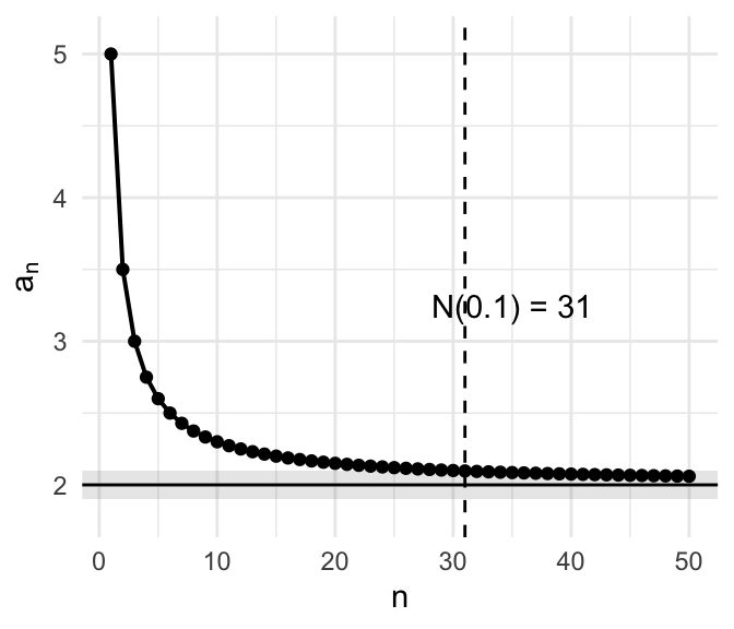
The number \(\epsilon\) represents an arbitrarily chosen tolerance around the candidate limit \(a\). The definition requires that, once \(n\) is sufficiently large, every subsequent element of the sequence lies within that tolerance. The threshold \(N(\epsilon)\) may depend on the chosen tolerance: a smaller value of \(\epsilon\) will generally require a larger value of \(N(\epsilon)\).

Convergence does not require the sequence to reach its limit at a finite value of \(n\), nor does it require the sequence to move monotonically toward the limit. It requires only that the entire tail of the sequence eventually remain arbitrarily close to the limit.

Example 3.1 (Convergence of a Scalar Sequence) Consider \(a_n=2+\frac{3}{n}\). The proposed limit is \(a=2\). For any \(\epsilon>0\), \[\begin{aligned} |a_n-2| = \left| 2+\frac{3}{n}-2 \right| = \frac{3}{n}. \end{aligned}\]

To ensure that \(|a_n-2|<\epsilon\), we require \(\frac{3}{n}<\epsilon\), which is equivalent to \(n>\frac{3}{\epsilon}\). One valid integer threshold is therefore \[N(\epsilon) = \left\lfloor\frac{3}{\epsilon}\right\rfloor+1,\] where for any real number \(x\), the floor function, denoted by \(\left\lfloor x\right\rfloor\) is the greatest integer less than or equal to \(x\). For every \(n\geq N(\epsilon)\), we then have \(|a_n-2|<\epsilon\). Hence, \[\lim_{n\to\infty} \left( 2+\frac{3}{n} \right) =2.\]

Figure 3.1 illustrates the definition using \(\epsilon=0.1\). In this case, a valid threshold is \(N(0.1)=31\). Every element of the sequence from \(n=31\) onward lies strictly between \(2-0.1\) and \(2+0.1\).

Figure 3.1: Convergence of the sequence \(a_n=2+3/n\) to 2

3.1.1 Sequences of Matrices

Econometric asymptotics frequently involve matrices whose entries change with the sample size. A sequence of matrices is simply an ordered collection \[\mathbf A_1,\mathbf A_2,\mathbf A_3,\ldots.\]

For convergence to a fixed matrix, the dimensions of \(\mathbf A_n\) must remain fixed as \(n\) changes. Matrices with dimensions that increase with \(n\) will be considered later using different concepts.

Example 3.2 (A Sequence of Matrices) Let \(\mathbf X_n\) be the \(n\times2\) matrix whose \(i\)th row is \((1,i)\). Thus, \[\mathbf X_n = \begin{pmatrix} 1 & 1\\ 1 & 2\\ \vdots & \vdots\\ 1 & n \end{pmatrix}.\]

Although the number of rows of \(\mathbf X_n\) increases with \(n\), the matrix \[\mathbf Y_n = \frac{1}{n}\mathbf X_n^{\top}\mathbf X_n\] is \(2\times2\) for every \(n\). The first three elements of the sequence \(\{\mathbf Y_n\}\) are \[\mathbf Y_1 = \begin{pmatrix} 1&1\\ 1&1 \end{pmatrix}, \qquad \mathbf Y_2 = \begin{pmatrix} 1&3/2\\ 3/2&5/2 \end{pmatrix}, \qquad \mathbf Y_3 = \begin{pmatrix} 1&2\\ 2&14/3 \end{pmatrix}.\]

For a general \(n\), \[\begin{aligned} \mathbf Y_n = \begin{pmatrix} 1 & \dfrac{1}{n}\displaystyle\sum_{i=1}^{n}i \\[6pt] \dfrac{1}{n}\displaystyle\sum_{i=1}^{n}i & \dfrac{1}{n}\displaystyle\sum_{i=1}^{n}i^2 \end{pmatrix} = \begin{pmatrix} 1 & \dfrac{n+1}{2} \\[6pt] \dfrac{n+1}{2} & \dfrac{(n+1)(2n+1)}{6} \end{pmatrix}. \end{aligned}\]

This example defines a valid sequence of fixed-dimensional matrices. It does not, however, converge to a finite matrix because three of its four entries grow without bound.

Definition 3.2 (Convergence of a Matrix Sequence) Let \(\{\mathbf A_n\}_{n=1}^{\infty}\) be a sequence of \(q\times k\) real matrices, where \(q\) and \(k\) do not depend on \(n\). The sequence converges to the \(q\times k\) matrix \(\mathbf A\) if \[[\mathbf A_n]_{ij} \to [\mathbf A]_{ij}\] for every \(i=1,\ldots,q\) and \(j=1,\ldots,k\).

Thus, convergence of a fixed-dimensional matrix sequence means convergence element by element. Every entry of \(\mathbf A_n\) must approach the corresponding entry of \(\mathbf A\).

3.1.2 Continuous Transformations of Convergent Sequences

Often the object of interest is not the original sequence itself, but a function of that sequence. Continuity ensures that limits can be passed through the function.

Definition 3.3 (Continuity) Let \(\mathbf g:\mathbb R^k\to\mathbb R^\ell\), and let \(\mathbf b\in\mathbb R^k\). The function \(\mathbf g\) is continuous at \(\mathbf b\) if, for every sequence \(\{\mathbf b_n\}\) satisfying \(\mathbf b_n\to\mathbf b\), \[\mathbf g(\mathbf b_n) \to \mathbf g(\mathbf b).\]

Equivalently, \(\mathbf g\) is continuous at \(\mathbf b\) if, for every \(\epsilon>0\), there exists a \(\delta>0\) such that \[\|\mathbf a-\mathbf b\|<\delta\] implies \[\|\mathbf g(\mathbf a)-\mathbf g(\mathbf b)\|<\epsilon.\]

The function is continuous on a set \(B\subseteq\mathbb R^k\) if it is continuous at every point in \(B\).

For example, if \(\mathbf a_n\to\mathbf a\) and \(\mathbf b_n\to\mathbf b\), then continuity of addition and multiplication implies \[\mathbf a_n+\mathbf b_n \to \mathbf a+\mathbf b\] and, for vectors of fixed dimensions, \[\mathbf a_n\mathbf b_n^{\top} \to \mathbf a\mathbf b^{\top}.\]

The matrix inverse is continuous at every nonsingular matrix. More precisely, if \(\mathbf A_n\to\mathbf A\) and \(\mathbf A\) is nonsingular, then \(\mathbf A_n\) is nonsingular for all sufficiently large \(n\) and \[\mathbf A_n^{-1} \to \mathbf A^{-1}.\]

To see why the nonsingularity condition matters, note that continuity of the determinant gives \[\det(\mathbf A_n) \to \det(\mathbf A).\]

If \(\det(\mathbf A)\neq0\), then \(\det(\mathbf A_n)\) must also be nonzero for all sufficiently large \(n\). A common econometric application is \[\frac{1}{n}\mathbf X^{\top}\mathbf X \to \mathbf Q,\] where \(\mathbf Q\) is finite and nonsingular. In that case, \[\left( \frac{1}{n}\mathbf X^{\top}\mathbf X \right)^{-1} \to \mathbf Q^{-1}.\]

3.1.3 Bounded Sequences

A sequence does not need to converge in order to remain within finite bounds.

Definition 3.4 (Bounded Sequence) A sequence of real numbers \(\{a_n\}_{n=1}^{\infty}\) is bounded if there exists a finite constant \(C\) such that \[|a_n|\leq C\] for every \(n\). If no such constant exists, the sequence is unbounded.

Every sequence that converges to a finite limit is bounded. The converse is not true. For example, \(a_n=(-1)^n\) is bounded because \(|a_n|=1\) for every \(n\), but it does not converge. By contrast, \(a_n=\frac{1}{n}\) is bounded and converges to zero.

Unboundedness should not be confused with divergence to positive infinity. We write \(a_n\to+\infty\) if, for every finite number \(M\), there exists an integer \(N(M)\) such that \(a_n>M\) for every \(n\geq N(M)\). Similarly, \(a_n\to-\infty\) if the sequence eventually falls below every finite lower bound. An unbounded sequence need not satisfy either condition. For example, \(a_n=(-1)^n n\) is unbounded but alternates between increasingly large positive and negative values, so it converges neither to \(+\infty\) nor to \(-\infty\).

Example 3.3 (Boundedness and Limits of Matrix Sequences) Consider again the sequence \(\{\mathbf Y_n\}\) from Example 3.2. Its \((1,1)\) entry is equal to one for every \(n\), but \[\frac{n+1}{2} \to +\infty\] and \[\frac{(n+1)(2n+1)}{6} \to +\infty.\]

The matrix sequence therefore has no finite elementwise limit. Now consider \[\mathbf A_n = \begin{pmatrix} 3n^{-1} & n^{-1}\\ 3 & 1+n^{-1} \end{pmatrix}.\]

Each entry has a finite limit: \[3n^{-1}\to0, \qquad n^{-1}\to0, \qquad 3\to3, \qquad 1+n^{-1}\to1.\]

Therefore, \[\mathbf A_n \to \begin{pmatrix} 0&0\\ 3&1 \end{pmatrix}.\]

3.1.4 Deterministic Orders of Magnitude

Sometimes the exact limit of a sequence is less important than its rate of growth or decline. Big-\(O\) and little-\(o\) notation provide a concise way to compare the magnitude of a sequence with a benchmark rate.

Definition 3.5 (Big-\(O\) and Little-\(o\)) Let \(\lambda\in\mathbb R\).

1. The sequence \(\{x_n\}\) is \(O(n^\lambda)\) if there exist finite constants \(C>0\) and \(N\) such that \(|x_n|\leq Cn^\lambda\) for every \(n\geq N\). Equivalently, \(x_n/n^\lambda\) is eventually bounded.

2. The sequence \(\{x_n\}\) is \(o(n^\lambda)\) if \(\frac{x_n}{n^\lambda} \to0\).

3. A fixed-dimensional vector or matrix sequence is \(O(n^\lambda)\) or \(o(n^\lambda)\) if the corresponding statement holds for every element.

The notation \(x_n=O(n^\lambda)\) provides an asymptotic upper bound: the magnitude of \(x_n\) grows no faster than a constant multiple of \(n^\lambda\). The stronger statement \(x_n=o(n^\lambda)\) means that \(x_n\) becomes negligible relative to \(n^\lambda\).

Two distinctions are important. First, \[x_n=o(n^\lambda) \quad\Longrightarrow\quad x_n=O(n^\lambda),\] because every sequence that converges to zero is bounded. Second, if \(x_n\to x\) for a finite \(x\), then \(x_n=O(1)\); however, \(x_n=o(1)\) only when \(x=0\).

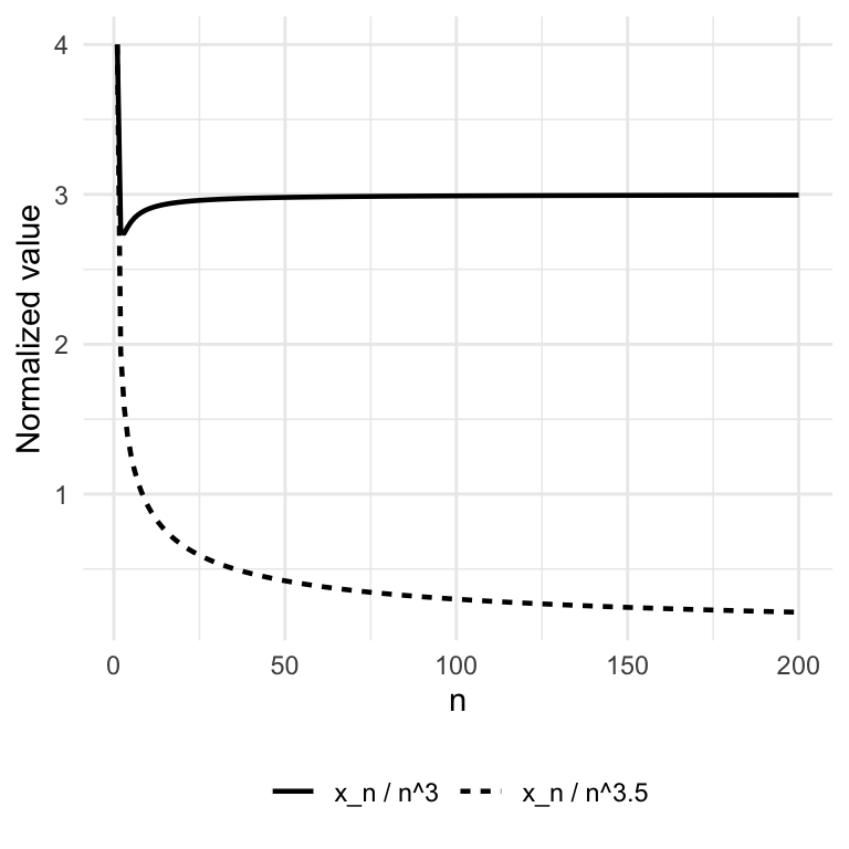
Example 3.4 (Orders of Magnitude) Consider \(x_n=3n^3-n^2+2\). Dividing by \(n^3\) gives \[\frac{x_n}{n^3} = 3-\frac{1}{n}+\frac{2}{n^3} \to3.\]

The normalized sequence is bounded, so \(x_n=O(n^3)\). Because its normalized limit is not zero, \(x_n\) is not \(o(n^3)\). For every \(\epsilon>0\), however, \[\begin{aligned} \frac{x_n}{n^{3+\epsilon}} = 3n^{-\epsilon} - n^{-1-\epsilon} + 2n^{-3-\epsilon} \to0. \end{aligned}\]

Therefore, \[x_n=o(n^{3+\epsilon}) \qquad \text{for every }\epsilon>0.\]

As a second example, let \(x_n=3+\frac{1}{n}\). Since \(x_n\to3\), the sequence is \(O(1)\) but not \(o(1)\). Nevertheless, for any \(\epsilon>0\), \[\frac{x_n}{n^\epsilon} = 3n^{-\epsilon}+n^{-1-\epsilon} \to0,\] so \(x_n=o(n^\epsilon)\).

Finally, consider \[\mathbf x_n = \begin{pmatrix} 3n^{-1}\\ n^{-1} \end{pmatrix}.\]

Both elements converge to zero. Hence, \(\mathbf x_n=o(1)\), which also implies \(\mathbf x_n=O(1)\).

Figure 3.2 illustrates the first case in Example 3.4. The sequence \(x_n/n^3\) remains bounded and approaches three. To make the distinction visually clear over a moderate range of \(n\), the second normalization uses \(\epsilon=0.5\); the sequence \(x_n/n^{3.5}\) approaches zero.

Figure 3.2: Big-\(O\) and little-\(o\) behavior of \(x_n=3n^3-n^2+2\)

The following proposition summarizes the basic algebra of deterministic orders.

Proposition 3.1 (Properties of Big-\(O\) and Little-\(o\)) Let \(a_n\) and \(b_n\) be scalar sequences, let \(\lambda,\mu\in\mathbb R\), and let \(\kappa=\max\{\lambda,\mu\}.\)

Then:

1. If \(a_n=O(n^\lambda)\) and \(b_n=O(n^\mu)\), then \(a_nb_n=O(n^{\lambda+\mu})\) and \(a_n+b_n=O(n^\kappa).\)

2. If \(a_n=o(n^\lambda)\) and \(b_n=o(n^\mu)\), then \(a_nb_n=o(n^{\lambda+\mu})\) and \(a_n+b_n=o(n^\kappa).\)

3. If \(a_n=O(n^\lambda)\) and \(b_n=o(n^\mu)\), then \(a_nb_n=o(n^{\lambda+\mu})\) and \(a_n+b_n=O(n^\kappa).\)

Proof. We prove each statement directly from Definition 3.5.

For the first product result, \(a_n=O(n^\lambda)\) and \(b_n=O(n^\mu)\) imply that there exist finite constants \(C_a,C_b>0\) and an integer \(N\) such that, for every \(n\geq N\), \[|a_n|\leq C_an^\lambda \qquad\text{and}\qquad |b_n|\leq C_bn^\mu.\]

Multiplying the two inequalities gives \[|a_nb_n| \leq C_aC_bn^{\lambda+\mu},\] so \(a_nb_n=O(n^{\lambda+\mu})\).

For the first sum result, \(\lambda\leq\kappa\) and \(\mu\leq\kappa\). Therefore, for every \(n\geq1\), \[n^\lambda\leq n^\kappa \qquad\text{and}\qquad n^\mu\leq n^\kappa.\]

Using the triangle inequality (see Definition 3.24), \[\begin{aligned} |a_n+b_n| &\leq |a_n|+|b_n| \\ &\leq C_an^\lambda+C_bn^\mu \\ &\leq (C_a+C_b)n^\kappa. \end{aligned}\]

Hence, \[a_n+b_n=O(n^\kappa).\]

For the second product result, write \[\frac{a_nb_n}{n^{\lambda+\mu}} = \left( \frac{a_n}{n^\lambda} \right) \left( \frac{b_n}{n^\mu} \right).\]

Both factors converge to zero. Their product therefore converges to zero, so \(a_nb_n=o(n^{\lambda+\mu})\).

For the second sum result, \[\frac{a_n+b_n}{n^\kappa} = \frac{a_n}{n^\kappa} + \frac{b_n}{n^\kappa}.\]

Consider the first term. It can be written as \[\frac{a_n}{n^\kappa} = \left( \frac{a_n}{n^\lambda} \right) n^{\lambda-\kappa}.\]

The first factor converges to zero. Because \(\lambda-\kappa\leq0\), the second factor is bounded by one for \(n\geq1\). Consequently, \[\frac{a_n}{n^\kappa} \to0.\]

The same argument gives \[\frac{b_n}{n^\kappa} \to0.\]

It follows that \[\frac{a_n+b_n}{n^\kappa} \to0,\] and therefore \(a_n+b_n=o(n^\kappa)\).

For the third product result, \[\frac{a_nb_n}{n^{\lambda+\mu}} = \left( \frac{a_n}{n^\lambda} \right) \left( \frac{b_n}{n^\mu} \right).\]

The first factor is bounded and the second converges to zero. The product thus converges to zero, which establishes \[a_nb_n=o(n^{\lambda+\mu}).\]

Finally, \(b_n=o(n^\mu)\) implies \(b_n=O(n^\mu)\). The first part of the proposition can therefore be applied to the sum of \(a_n\) and \(b_n\), yielding \[a_n+b_n=O(n^\kappa).\]

This completes the proof.

3.2 Convergence in Probability

The previous section considered deterministic sequences. For such a sequence, once the index is sufficiently large, every subsequent element must remain within any prescribed distance of its limit. Econometric estimators, however, are random variables because their values depend on the particular sample that is observed. Even with a large sample, an estimator can occasionally be far from the parameter it is intended to estimate.

For a sequence of random variables, it is therefore inappropriate to require that the distance from the limit be smaller than a given tolerance in every possible sample. Instead, we require the probability of a discrepancy larger than that tolerance to become arbitrarily small as the sample size increases. This idea leads to convergence in probability.

Definition 3.6 (Convergence in Probability) A sequence of random variables \(\{X_n\}_{n=1}^{\infty}\) converges in probability to a random variable \(X\) if, for every \(\epsilon>0\), \[\lim_{n\to\infty} \Pr\left( |X_n-X|>\epsilon \right) =0.\]

We write \[X_n\overset{p}{\longrightarrow}X.\]

When the limit is a constant \(\alpha\), it is called the probability limit of \(X_n\), and we may write \[\operatorname{plim}_{n\to\infty}X_n=\alpha\] or simply \[\operatorname{plim}X_n=\alpha.\]

The event \(|X_n-X|>\epsilon\) occurs when \(X_n\) lies outside an interval of radius \(\epsilon\) around its limit. Convergence in probability requires the probability of this event to approach zero. Equivalently, \[\lim_{n\to\infty} \Pr\left( |X_n-X|\leq\epsilon \right) =1.\]

Thus, convergence in probability does not say that \(X_n\) must be close to \(X\) in every sample. It says that, for any fixed tolerance, samples in which the discrepancy exceeds that tolerance become increasingly unlikely.

When the limit is a constant \(\alpha\), \[X_n\overset{p}{\longrightarrow}\alpha\] if and only if \[X_n-\alpha\overset{p}{\longrightarrow}0.\]

Figure 3.3 illustrates this idea using \[X_n=\alpha+\frac{Z}{\sqrt{n}}, \qquad Z\sim\mathcal N(0,1).\]

For every \(n\), the distribution is centered at \(\alpha\), but its variance is \(1/n\). As \(n\) grows, the distribution becomes increasingly concentrated around \(\alpha\), and the probability mass outside the fixed interval \([\alpha-\epsilon,\alpha+\epsilon]\) approaches zero.

Figure 3.3: Concentration of \(X_n\) around its probability limit

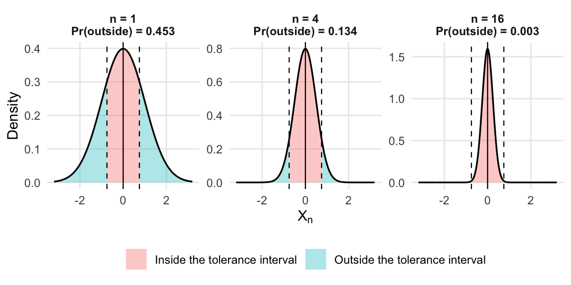
The interval in the figure remains fixed as \(n\) changes. What changes is the distribution of \(X_n\). Convergence occurs because an increasing share of the distribution lies inside the interval, not because the tolerance itself is made larger.

3.2.1 Random Vectors and Matrices

The definition of convergence in probability extends naturally to random vectors. Let \(\mathbf X_n\) and \(\mathbf X\) be \(k\times1\) random vectors, where \(k\) is fixed.

Definition 3.7 (Convergence in Probability for Random Vectors) The sequence \(\{\mathbf X_n\}\) converges in probability to \(\mathbf X\) if, for every \(\epsilon>0\), \[\lim_{n\to\infty} \Pr\left( \|\mathbf X_n-\mathbf X\|>\epsilon \right) =0,\] where \(\|\cdot\|\) denotes the Euclidean norm.

If \[\mathbf X_n = \begin{pmatrix} X_{1n}\\ \vdots\\ X_{kn} \end{pmatrix}, \qquad \mathbf X = \begin{pmatrix} X_1\\ \vdots\\ X_k \end{pmatrix},\] then \[\|\mathbf X_n-\mathbf X\| = \left[ \sum_{j=1}^{k}(X_{jn}-X_j)^2 \right]^{1/2}.\]

Because the dimension \(k\) is fixed, vector convergence in probability is equivalent to convergence in probability of every component.

Proposition 3.2 (Componentwise Characterization) For fixed \(k\), \[\mathbf X_n\overset{p}{\longrightarrow}\mathbf X\] if and only if \[X_{jn}\overset{p}{\longrightarrow}X_j \qquad \text{for every }j=1,\ldots,k.\]

For a sequence of random matrices with fixed dimensions, convergence in probability is defined element by element. If \(\mathbf A_n\) and \(\mathbf A\) are \(q\times k\) matrices, then \[\mathbf A_n\overset{p}{\longrightarrow}\mathbf A\] means \[A_n[i,j]\overset{p}{\longrightarrow}A[i,j]\] for every \(i=1,\ldots,q\) and \(j=1,\ldots,k\). Because the number of entries is fixed, this is equivalent to convergence under any standard matrix norm.

3.2.2 Continuous Transformations

A common econometric problem is to determine the probability limit of a function of an estimator. Expectations generally do not pass through nonlinear functions. For example, \[\mathbb E\left[ \exp(X) \right] \neq \exp\left( \mathbb E[X] \right)\] in general. Probability limits behave differently: continuous transformations can be applied after taking the probability limit.

Theorem 3.1 (Continuous Mapping Theorem) Let \(\mathbf X_n\) be a sequence of \(k\times1\) random vectors such that \[\mathbf X_n\overset{p}{\longrightarrow}\mathbf a,\] where \(\mathbf a\in\mathbb R^k\) is constant. If \(\mathbf g:\mathbb R^k\rightarrow\mathbb R^m\) is continuous at \(\mathbf a\), then \[\mathbf g(\mathbf X_n) \overset{p}{\longrightarrow} \mathbf g(\mathbf a).\]

Equivalently, \[\operatorname{plim}\mathbf g(\mathbf X_n) = \mathbf g\left( \operatorname{plim}\mathbf X_n \right).\]

Proof. Let \(\epsilon>0\). Since \(\mathbf g\) is continuous at \(\mathbf a\), there exists \(\delta>0\) such that \(\|\mathbf x-\mathbf a\|<\delta\) implies \(\|\mathbf g(\mathbf x)-\mathbf g(\mathbf a)\|<\epsilon\) (see Definition 3.3). Therefore, if \(\|\mathbf g(\mathbf X_n)-\mathbf g(\mathbf a)\|\geq\epsilon\), then it must be the case that \(\|\mathbf X_n-\mathbf a\|\geq\delta\). Therefore, the corresponding events satisfy \[ \left\lbrace |\mathbf g(\mathbf X_n)-\mathbf g(\mathbf a)|\geq \epsilon\right\rbrace \subseteq \left\lbrace|\mathbf X_n-\mathbf a|\geq \delta \right\rbrace. \]

Since the probability of a subset cannot exceed the probability of the set that contains it \((A\subseteq B\Longrightarrow \Pr(A)\leq \Pr(B))\), \[ \Pr\left( |\mathbf g(\mathbf X_n)-\mathbf g(\mathbf a)|\geq\epsilon \right) \leq \Pr\left( |\mathbf X_n-\mathbf a|\geq\delta \right). \]

Because \(\mathbf X_n\overset{p}{\longrightarrow}\mathbf a\), the probability on the right converges to zero. Hence \(\mathbf g(\mathbf X_n)\overset{p}{\longrightarrow}\mathbf g(\mathbf a)\).

The continuity requirement is essential. For example, the reciprocal function \(g(x)=1/x\) is continuous at every nonzero value but is not continuous at zero. Thus, if \(X_n\overset{p}{\longrightarrow}c\) with \(c\neq0\), then \[\frac{1}{X_n} \overset{p}{\longrightarrow} \frac{1}{c}.\]

Clearly, Theorem 3.1 cannot be applied to the reciprocal when the probability limit is zero.

3.2.3 Consistent Estimators

Convergence in probability provides the standard definition of consistency in econometrics.

Definition 3.8 (Consistent Estimator) Let \(\widehat{\boldsymbol\theta}_n\) be an estimator of a fixed parameter vector \(\boldsymbol\theta_0\). The estimator is consistent for \(\boldsymbol\theta_0\) if \[\widehat{\boldsymbol\theta}_n \overset{p}{\longrightarrow} \boldsymbol\theta_0.\]

Equivalently, \[\operatorname{plim} \widehat{\boldsymbol\theta}_n = \boldsymbol\theta_0.\]

Consistency is a property of a sequence of estimators indexed by the sample size, not of a single numerical estimate. It means that, for any fixed neighborhood of the true parameter, the probability that the estimator lies outside that neighborhood approaches zero as the sample size increases. Consistency does not require the estimator to be unbiased in finite samples, and it does not describe how quickly the estimator approaches the parameter.

Convergence in probability is sometimes called weak convergence in probability, and consistency based on it is called weak consistency. In econometrics, the qualifier “weak” is usually omitted unless a distinction from almost sure convergence is needed.

Example 3.5 (Consistency of the OLS Estimator) Consider the linear regression model \[\mathbf y = \mathbf X\boldsymbol\beta_0 + \boldsymbol\varepsilon,\] where \(\mathbf X\) is an \(n\times k\) regressor matrix and \(\boldsymbol\beta_0\) is a fixed \(k\times1\) parameter vector. Suppose that \[\frac{1}{n} \mathbf X^{\top}\boldsymbol\varepsilon \overset{p}{\longrightarrow} \mathbf 0\] and \[\frac{1}{n} \mathbf X^{\top}\mathbf X \overset{p}{\longrightarrow} \mathbf Q,\] where \(\mathbf Q\) is finite and positive definite.

Whenever \(\mathbf X^{\top}\mathbf X\) is nonsingular, the OLS estimator satisfies \[\begin{aligned} \widehat{\boldsymbol\beta}_n &= \left( \mathbf X^{\top}\mathbf X \right)^{-1} \mathbf X^{\top}\mathbf y = \boldsymbol\beta_0 + \left( \frac{1}{n} \mathbf X^{\top}\mathbf X \right)^{-1} \left( \frac{1}{n} \mathbf X^{\top}\boldsymbol\varepsilon \right). \end{aligned} \tag{3.1}\]

Because \(\mathbf Q\) is positive definite, it is nonsingular. Matrix inversion is continuous at every nonsingular matrix, so the Theorem 3.1 gives \[\left( \frac{1}{n} \mathbf X^{\top}\mathbf X \right)^{-1} \overset{p}{\longrightarrow} \mathbf Q^{-1}.\]

More explicitly, continuity of the determinant implies \[\det\left( \frac{1}{n} \mathbf X^{\top}\mathbf X \right) \overset{p}{\longrightarrow} \det(\mathbf Q)>0.\]

Therefore, \[\Pr\left[ \det\left( \frac{1}{n} \mathbf X^{\top}\mathbf X \right)>0 \right] \longrightarrow1,\] so the inverse exists with probability approaching one. Applying the product rule for probability limits to Equation 3.1 yields \[\begin{aligned} \widehat{\boldsymbol\beta}_n &\overset{p}{\longrightarrow} \boldsymbol\beta_0 + \mathbf Q^{-1}\mathbf 0 \\ &= \boldsymbol\beta_0. \end{aligned}\]

Thus, the OLS estimator is consistent under the stated assumptions.

In Example 3.5 the condition \[\frac{1}{n} \mathbf X^{\top}\boldsymbol\varepsilon \overset{p}{\longrightarrow} \mathbf 0\] controls the asymptotic relation between the regressors and the disturbances, whereas positive definiteness of \(\mathbf Q\) guarantees sufficient asymptotic variation and absence of perfect collinearity.

3.2.4 Almost Sure Convergence

Convergence in probability allows the event \(|X_n-X|>\epsilon\) to occur at arbitrarily large values of \(n\), provided its probability becomes small. Almost sure convergence imposes a stronger, pathwise requirement: except on an event of probability zero, every realized sequence must eventually remain arbitrarily close to its limit.

Definition 3.9 (Almost Sure Convergence) A sequence of random variables \(\{X_n\}\) converges almost surely to a random variable \(X\) if \[\Pr\left( \lim_{n\to\infty}X_n=X \right) =1.\]

We write \[X_n\overset{a.s.}{\longrightarrow}X.\]

Equivalently, for every \(\epsilon>0\), \[\Pr\left( |X_n-X|>\epsilon \text{ infinitely often} \right) =0.\]

The phrase “infinitely often” means that the inequality occurs for infinitely many values of \(n\). Therefore, almost sure convergence says that, with probability one, for every tolerance \(\epsilon>0\) there is a sample-path-specific index after which all subsequent values lie within that tolerance.

Proposition 3.3 (Almost Sure Convergence Implies Convergence in Probability) If \(X_n\overset{a.s.}{\longrightarrow}X,\) then \(X_n\overset{p}{\longrightarrow}X.\)

The converse is not true in general: convergence in probability does not necessarily imply almost sure convergence.

3.2.5 Convergence in Quadratic Mean

Convergence in quadratic mean measures the expected squared distance between two random variables. It is stronger than convergence in probability, but it is often easier to verify because it can be studied using means, variances, and covariances.

Definition 3.10 (Convergence in Quadratic Mean) A sequence of random variables \(\{X_n\}\) converges in quadratic mean to a random variable \(X\) if the relevant second moments exist and \[\lim_{n\to\infty} \mathbb E\left[ (X_n-X)^2 \right] =0.\]

We write \[X_n\overset{q.m.}{\longrightarrow}X.\]

When the limit is a constant \(c\), the mean squared error admits the familiar bias–variance decomposition: \[\begin{aligned} \mathbb E\left[ (X_n-c)^2 \right] &= \operatorname{Var}(X_n) + \left[ \mathbb E(X_n)-c \right]^2. \end{aligned} \tag{3.2}\]

Consequently, convergence of the mean to \(c\) together with convergence of the variance to zero is sufficient for quadratic-mean convergence.

Proposition 3.4 (Mean and Variance Condition) Suppose \(X_n\) has finite mean \(\mu_n\) and finite variance \(\sigma_n^2\). If \(\mu_n\to c\) and \(\sigma_n^2\to0,\) then \(X_n\overset{q.m.}{\longrightarrow}c.\)

Proof. By Equation 3.2, \[\mathbb E\left[ (X_n-c)^2 \right] = \sigma_n^2 + (\mu_n-c)^2.\]

The first term converges to zero by assumption. Since \(\mu_n\to c\), the second term also converges to zero. Therefore, \[\mathbb E\left[ (X_n-c)^2 \right] \to0,\] which is the definition of convergence in quadratic mean.

Theorem 3.2 (Quadratic-Mean Convergence Implies Convergence in Probability) If \(X_n\overset{q.m.}{\longrightarrow}X,\) then \(X_n\overset{p}{\longrightarrow}X.\)

Proof. For every \(\epsilon>0\), Markov’s inequality (Theorem 3.27) applied to the nonnegative random variable \((X_n-X)^2\) gives \[\begin{aligned} \Pr\left( |X_n-X|>\epsilon \right) &= \Pr\left( (X_n-X)^2>\epsilon^2 \right) \\ &\leq \frac{ \mathbb E\left[(X_n-X)^2\right] }{ \epsilon^2 }. \end{aligned}\]

Quadratic-mean convergence implies that the numerator on the right converges to zero. Hence \[\Pr\left( |X_n-X|>\epsilon \right) \to0,\] which establishes convergence in probability.

The converse is not generally true. A sequence can converge in probability while its second moments fail to converge appropriately or fail to exist.

3.2.5.1 Random Vectors

For a fixed-dimensional random vector, quadratic-mean convergence is defined using squared Euclidean distance.

Definition 3.11 (Quadratic-Mean Convergence for Random Vectors) Let \(\widehat{\boldsymbol\theta}_n\) and \(\boldsymbol\theta_0\) be \(k\times1\) random vectors, where \(k\) is fixed. We say that \[\widehat{\boldsymbol\theta}_n \overset{q.m.}{\longrightarrow} \boldsymbol\theta_0\] if \[\mathbb E\left[ \left\| \widehat{\boldsymbol\theta}_n- \boldsymbol\theta_0 \right\|^2 \right] \to0.\]

When \(\boldsymbol\theta_0\) is a fixed parameter vector, \[\begin{aligned} \mathbb E\left[ \left( \widehat{\boldsymbol\theta}_n- \boldsymbol\theta_0 \right)^{\top} \left( \widehat{\boldsymbol\theta}_n- \boldsymbol\theta_0 \right) \right] = \left \| \mathbb E\left( \widehat{\boldsymbol\theta}_n \right) - \boldsymbol\theta_0 \right\|^2 + \operatorname{tr}\left[ \operatorname{Var}\left( \widehat{\boldsymbol\theta}_n \right) \right]. \end{aligned} \tag{3.3}\]

To see the decomposition, write \[\widehat{\boldsymbol\theta}_n- \boldsymbol\theta_0 = \left[ \widehat{\boldsymbol\theta}_n- \mathbb E\left( \widehat{\boldsymbol\theta}_n \right) \right] + \left[ \mathbb E\left( \widehat{\boldsymbol\theta}_n \right) - \boldsymbol\theta_0 \right].\]

After expanding the squared norm, the cross term has expectation zero because \[\mathbb E\left[ \widehat{\boldsymbol\theta}_n- \mathbb E\left( \widehat{\boldsymbol\theta}_n \right) \right] = \mathbf 0.\]

The expected squared Euclidean norm of an estimator centered at its expectation equals the trace of its covariance matrix.¹ Therefore, for fixed \(k\), asymptotic unbiasedness together with a covariance matrix that converges to the zero matrix is sufficient for quadratic-mean convergence and hence for consistency.

Theorem 3.3 (Consistency of the Sample Mean) Let \(X_1,\ldots,X_n\) be an independent and identically distributed random sample with \(\mathbb E(X_i)=\mu\) and \(\operatorname{Var}(X_i)=\sigma^2<\infty.\) Then the sample mean \[\overline X_n = \frac{1}{n} \sum_{i=1}^{n}X_i \] is a consistent estimator of \(\mu\).

Proof. Independence and identical distribution imply \(\mathbb E(\overline X_n)=\mu\) and \[\begin{aligned} \operatorname{Var}(\overline X_n) &= \operatorname{Var}\left( \frac{1}{n} \sum_{i=1}^{n}X_i \right) \\ &= \frac{1}{n^2} \sum_{i=1}^{n} \operatorname{Var}(X_i) \\ &= \frac{\sigma^2}{n} \\ &\to0. \end{aligned}\]

Using the bias–variance decomposition, \[\begin{aligned} \mathbb E\left[ (\overline X_n-\mu)^2 \right] &= \operatorname{Var}(\overline X_n) + \left[ \mathbb E(\overline X_n)-\mu \right]^2 \\ &= \frac{\sigma^2}{n} \\ &\to0. \end{aligned}\]

Thus, \[\overline X_n \overset{q.m.}{\longrightarrow} \mu.\]

Since quadratic-mean convergence implies convergence in probability, \[\overline X_n \overset{p}{\longrightarrow} \mu.\]

The argument above is the finite-variance weak law of large numbers. A more general treatment of laws of large numbers is given in the next section.

Theorem 3.4 (A Mean–Variance Condition for Consistency) Let \(\widehat\theta_n\) be a scalar estimator of \(\theta_0\). If \(\mathbb E(\widehat\theta_n) \to \theta_0\) and \(\operatorname{Var}(\widehat\theta_n) \to0,\) then \[\widehat\theta_n \overset{p}{\longrightarrow} \theta_0. \]

Proof. For every \(\epsilon>0\), Markov’s inequality (Theorem 3.27) gives \[\Pr\left( |\widehat\theta_n-\theta_0|>\epsilon \right) \leq \frac{ \mathbb E\left[ (\widehat\theta_n-\theta_0)^2 \right] }{ \epsilon^2 }.\]

Using the bias–variance decomposition, \[\mathbb E\left[ (\widehat\theta_n-\theta_0)^2 \right] = \operatorname{Var}(\widehat\theta_n) + \left[ \mathbb E(\widehat\theta_n)-\theta_0 \right]^2.\]

Both terms on the right converge to zero by assumption. Consequently, \[\Pr\left( |\widehat\theta_n-\theta_0|>\epsilon \right) \to0,\] which proves consistency.

The theorem requires asymptotic unbiasedness, not exact unbiasedness at every sample size. It is only a sufficient condition. An estimator may be consistent even if its finite-sample bias does not vanish quickly enough for this particular argument to be convenient, and some consistent estimators do not possess finite second moments.

Example 3.6 (Sample Variance under Normal Sampling) For an independent normal sample, let \[s_n^2 = \frac{1}{n-1} \sum_{i=1}^{n} (X_i-\overline X_n)^2.\]

Then \(\mathbb E(s_n^2)=\sigma^2\) and \[\operatorname{Var}(s_n^2) = \frac{2\sigma^4}{n-1} \to0.\]

Therefore, \[s_n^2\overset{p}{\longrightarrow}\sigma^2.\]

Example 3.7 (Bernoulli Sample Mean) If \(X_i\) is Bernoulli with success probability \(\theta\), then \(\mathbb E(\overline X_n)=\theta\) and \[\operatorname{Var}(\overline X_n) = \frac{\theta(1-\theta)}{n} \to0.\]

Hence, \[\overline X_n \overset{p}{\longrightarrow} \theta.\]

3.2.6 Rules for Probability Limits

The continuous mapping theorem produces the familiar algebraic rules for probability limits. These rules are used repeatedly when establishing the consistency of econometric estimators.

Theorem 3.5 (Rules for Probability Limits) Suppose \(X_n\overset{p}{\longrightarrow}c\) and \(Y_n\overset{p}{\longrightarrow}d,\) where \(c\) and \(d\) are constants. Then:

1. Sum rule: \(X_n+Y_n \overset{p}{\longrightarrow} c+d.\)

2. Product rule: \(X_nY_n \overset{p}{\longrightarrow} cd.\)

3. Ratio rule: If \(d\neq0\), then \(\frac{X_n}{Y_n} \overset{p}{\longrightarrow} \frac{c}{d}.\)

For fixed-dimensional random matrices, suppose \(\mathbf A_n\overset{p}{\longrightarrow}\mathbf A\) and \(\mathbf B_n\overset{p}{\longrightarrow}\mathbf B.\)

Then:

4. Matrix product rule

   If the dimensions are conformable, \[ \mathbf A_n\mathbf B_n \overset{p}{\longrightarrow} \mathbf A\mathbf B. \]

5. Matrix inverse rule

   If \(\mathbf A\) is nonsingular, then \[\mathbf A_n^{-1} \overset{p}{\longrightarrow} \mathbf A^{-1},\] where \(\mathbf A_n^{-1}\) exists with probability approaching one.

Proof. First, scalar convergence of \(X_n\) and \(Y_n\) implies joint convergence: \[\begin{pmatrix} X_n\\ Y_n \end{pmatrix} \overset{p}{\longrightarrow} \begin{pmatrix} c\\ d \end{pmatrix}.\]

Indeed, for every \(\epsilon>0\), if \[|X_n-c|\leq\frac{\epsilon}{\sqrt2}\] and \[|Y_n-d|\leq\frac{\epsilon}{\sqrt2},\] then \[(X_n-c)^2+(Y_n-d)^2 \leq \epsilon^2.\]

Therefore, \[\begin{aligned} \Pr\left[ \left \| \begin{pmatrix} X_n\\ Y_n \end{pmatrix} - \begin{pmatrix} c\\ d \end{pmatrix} \right\|>\epsilon \right] \leq \Pr\left( |X_n-c|>\frac{\epsilon}{\sqrt2} \right) + \Pr\left( |Y_n-d|>\frac{\epsilon}{\sqrt2} \right), \end{aligned}\] and the right-hand side converges to zero.

The functions \(g_1(x,y)=x+y\) and \(g_2(x,y)=xy\) are continuous everywhere. Applying the continuous mapping theorem (Theorem 3.1) gives the sum and product rules.

The function \(g_3(x,y)=\frac{x}{y}\) is continuous at \((c,d)\) whenever \(d\neq0\). The continuous mapping theorem therefore gives the ratio rule.

For fixed matrix dimensions, every entry of \(\mathbf A_n\mathbf B_n\) is a finite sum of products of entries of \(\mathbf A_n\) and \(\mathbf B_n\). The scalar sum and product rules therefore imply \[\mathbf A_n\mathbf B_n \overset{p}{\longrightarrow} \mathbf A\mathbf B.\]

Finally, matrix inversion is continuous at every nonsingular matrix. If \(\mathbf A\) is nonsingular, the continuous mapping theorem gives \[\mathbf A_n^{-1} \overset{p}{\longrightarrow} \mathbf A^{-1}.\]

Continuity of the determinant also implies that \(\mathbf A_n\) is nonsingular with probability approaching one.

Example 3.8 (Probability Limit of a Linear Transformation) Let \[\mathbf A = \begin{pmatrix} 2&1\\ 1&1 \end{pmatrix}\] and suppose \[\mathbf X_n \overset{p}{\longrightarrow} \begin{pmatrix} 2\\ 5 \end{pmatrix}.\]

Then \[\begin{aligned} \mathbf A\mathbf X_n \overset{p}{\longrightarrow} \mathbf A \begin{pmatrix} 2\\ 5 \end{pmatrix} = \begin{pmatrix} 9\\ 7 \end{pmatrix}. \end{aligned}\]

Example 3.9 (Probability Limits of Matrix Functions) Suppose \[\mathbf Y_n \overset{p}{\longrightarrow} \begin{pmatrix} 1&2\\ 2&1 \end{pmatrix}\] and \[\mathbf X_n \overset{p}{\longrightarrow} \begin{pmatrix} 3&1\\ 2&1 \end{pmatrix}.\]

The product rule gives \[\begin{aligned} \mathbf X_n\mathbf Y_n &\overset{p}{\longrightarrow} \begin{pmatrix} 3&1\\ 2&1 \end{pmatrix} \begin{pmatrix} 1&2\\ 2&1 \end{pmatrix} \\ &= \begin{pmatrix} 5&7\\ 4&5 \end{pmatrix}. \end{aligned}\]

Because \[\det \begin{pmatrix} 3&1\\ 2&1 \end{pmatrix} =1\neq0,\] the inverse rule applies. Since \[\begin{pmatrix} 3&1\\ 2&1 \end{pmatrix}^{-1} = \begin{pmatrix} 1&-1\\ -2&3 \end{pmatrix},\] we obtain \[\begin{aligned} \mathbf X_n^{-1}\mathbf Y_n \overset{p}{\longrightarrow} \begin{pmatrix} 1&-1\\ -2&3 \end{pmatrix} \begin{pmatrix} 1&2\\ 2&1 \end{pmatrix} = \begin{pmatrix} -1&1\\ 4&-1 \end{pmatrix}. \end{aligned}\]

3.3 Law of Large Numbers

A large part of asymptotic econometrics consists of studying sample averages. Estimators and estimating equations are commonly constructed from expressions such as \[\frac{1}{n}\sum_{i=1}^{n}X_i, \qquad \frac{1}{n}\sum_{i=1}^{n}\mathbf x_i\mathbf x_i^{\top}, \qquad \frac{1}{n}\sum_{i=1}^{n}\mathbf x_i\varepsilon_i.\]

A law of large numbers provides conditions under which an average of random variables becomes close, in probability, to the corresponding average of its expectations. These results are central to econometrics because they allow us to establish probability limits without working directly from the definition of convergence in probability each time.

The preceding section proved that an i.i.d. sample mean is consistent when the observations have a finite variance. The first result below is stronger in one important respect: for identically distributed observations, it requires only a finite first absolute moment.

3.3.1 The i.i.d. Case

Theorem 3.6 (Khinchine’s Weak Law of Large Numbers) Let \(X_1,X_2,\ldots\) be independent and identically distributed random variables satisfying \(\mathbb E|X_i|<\infty\), and define \[\mu=\mathbb E(X_i), \qquad \overline X_n = \frac{1}{n}\sum_{i=1}^{n}X_i.\]

Then \[\overline X_n \overset{p}{\longrightarrow} \mu.\]

Equivalently, for every \(\epsilon>0\), \[\Pr\left( |\overline X_n-\mu|>\epsilon \right) \longrightarrow0.\]

The assumption \(\mathbb E|X_i|<\infty\) guarantees that the population mean is well defined and finite. The theorem does not require a finite variance or any higher-order moment.

The theorem says that averaging independent observations from the same population eliminates sampling variation in the limit. It does not say that every realized sample mean moves monotonically toward \(\mu\), nor that a sample mean must be close to \(\mu\) in every finite sample. It says that, for any fixed tolerance, the probability of a discrepancy larger than that tolerance tends to zero.

Example 3.10 (A Ratio of Sample Moments) Let \(X_1,X_2,\ldots\) be i.i.d. with \(\mathbb E(X_i)=\mu\), and \(\operatorname{Var}(X_i)=\sigma^2>0\), and suppose \(\mathbb E(X_i^2)<\infty\). Define \(s_n^2 =\frac{1}{n}\sum_{i=1}^{n}(X_i-\overline X_n)^2\). We want to find the probability limit of \[\widehat\theta_n = \frac{\overline X_n^2}{s_n^2}.\]

The WLLN (Theorem 3.6) gives \[\overline X_n \overset{p}{\longrightarrow} \mu\] and \[\frac{1}{n}\sum_{i=1}^{n}X_i^2 \overset{p}{\longrightarrow} \mathbb E(X_i^2).\]

Using \[s_n^2 = \frac{1}{n}\sum_{i=1}^{n}X_i^2 - \overline X_n^2,\] we obtain \[\begin{aligned} s_n^2 \overset{p}{\longrightarrow} \mathbb E(X_i^2)-\mu^2 = \sigma^2. \end{aligned}\]

Since \(\sigma^2>0\), the ratio rule in Theorem 3.5 yields \[\widehat\theta_n \overset{p}{\longrightarrow} \frac{\mu^2}{\sigma^2}.\]

This example illustrates a common econometric strategy. First, use an LLN to find the probability limits of the underlying sample moments. Then apply the rules for probability limits to obtain the limit of the estimator constructed from those moments.

3.3.2 Two Illustrations

The following examples use running averages. They show how a single realized sequence may stabilize as the number of observations increases. A single path is only an illustration: convergence in probability is a statement about the probability distribution across repeated samples, not about one particular realization.

Example 3.11 (Running Mean of Normal Observations) Suppose \[X_i \overset{\mathrm{i.i.d.}}{\sim} \mathcal N(1,0.5^2).\]

One infinite sequence \(X_1,X_2,\ldots\) generates the nested sample means \[\begin{aligned} \overline X_1 &= X_1, \\ \overline X_2 &= \frac{X_1+X_2}{2}, \\ \overline X_3 &= \frac{X_1+X_2+X_3}{3}, \\ &\ \vdots \\ \overline X_n &= \frac{1}{n}\sum_{i=1}^{n}X_i. \end{aligned}\]

Because \(\mathbb E(X_i)=1\), Khinchine’s WLLN implies \[\overline X_n \overset{p}{\longrightarrow} 1.\]

Figure 3.4: A running sample mean from a normal population

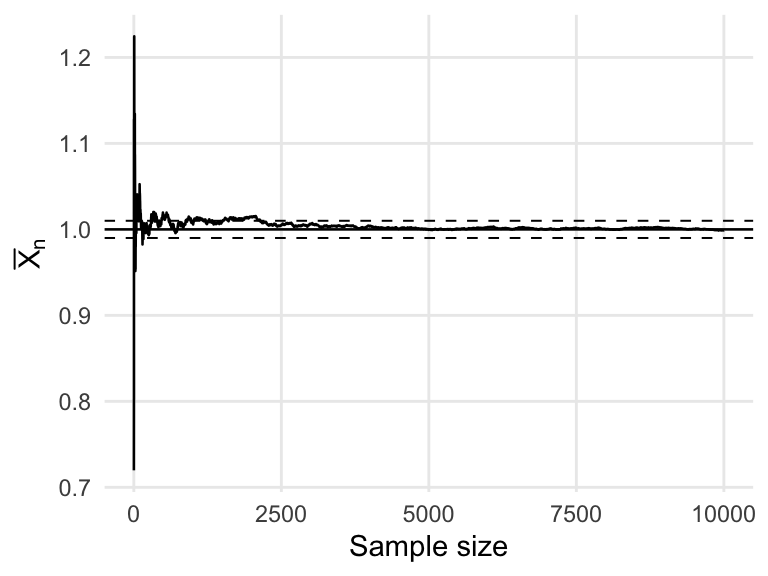
In Figure 3.4, the running mean fluctuates considerably when the sample is small because each new observation has a substantial influence on the average. As \(n\) grows, the contribution of any single observation is smaller, and the running mean settles near the population mean. The dashed lines show a tolerance interval of radius \(0.01\) around \(1\).

Example 3.12 (Tossing a Fair Coin) Let \[H_i = \begin{cases} 1, & \text{if toss }i\text{ produces heads},\\ 0, & \text{if toss }i\text{ produces tails}. \end{cases}\]

For a fair coin, \[H_i \overset{\mathrm{i.i.d.}}{\sim} \operatorname{Bernoulli}\left(\frac{1}{2}\right),\] so \[\mathbb E(H_i)=\frac{1}{2}.\]

The sample mean \[\overline H_n = \frac{1}{n}\sum_{i=1}^{n}H_i\] is the proportion of heads observed in the first \(n\) tosses. The WLLN implies \[\overline H_n \overset{p}{\longrightarrow} \frac{1}{2}.\]

Figure 3.5: Running proportion of heads in repeated tosses of a fair coin

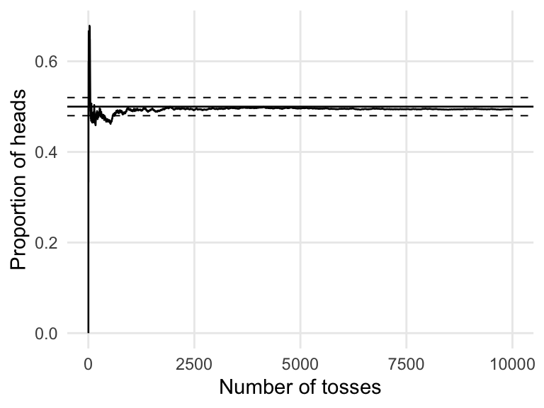
The proportion in Figure 3.5 may move far from \(1/2\) during the first few tosses. This does not contradict the WLLN. The theorem concerns the behavior of the proportion as the number of tosses becomes large. The dashed lines correspond to a tolerance of \(\epsilon=0.02\).

3.3.3 Transformations of i.i.d. Observations

Econometric sample moments are often averages of transformations of the original observations. For example, OLS involves averages of \(\mathbf x_i\mathbf x_i^{\top}\) and \(\mathbf x_i\varepsilon_i\), rather than averages of \(\mathbf x_i\) and \(\varepsilon_i\) separately. We therefore need to know when the i.i.d. property is preserved by a transformation.

Proposition 3.5 (Measurable Transformations Preserve the i.i.d. Property) Let \(\{\mathbf Z_i\}_{i=1}^{\infty}\) be an i.i.d. sequence of random vectors, and let \(\mathbf g\) be the same measurable function for every observation. Then \(\{\mathbf g(\mathbf Z_i)\}_{i=1}^{\infty}\) is also an i.i.d. sequence.

Continuity is not required for this result. Measurability is sufficient because it guarantees that events involving \(\mathbf g(\mathbf Z_i)\) have well-defined probabilities. For example, if \[\left\{ (\mathbf z_i^{\top},\mathbf x_i^{\top},\varepsilon_i)^{\top} \right\}_{i=1}^{\infty}\] is i.i.d., then each of the following sequences is i.i.d.: \[\left\{ \mathbf x_i\mathbf x_i^{\top} \right\}, \qquad \left\{ \mathbf x_i\varepsilon_i \right\}, \qquad \left\{ \mathbf z_i\mathbf x_i^{\top} \right\}, \qquad \left\{ \mathbf z_i\varepsilon_i \right\}, \qquad \left\{ \mathbf z_i\mathbf z_i^{\top} \right\}.\]

Preservation of the i.i.d. property does not by itself guarantee that an LLN can be applied. The relevant transformed variables must also satisfy the moment condition required by the theorem.

3.3.4 Application: OLS under Random Sampling

The abstract consistency argument for OLS in Example 3.5 assumed that \[\frac{1}{n}\mathbf X^{\top}\mathbf X \overset{p}{\longrightarrow} \mathbf Q\] and \[\frac{1}{n}\mathbf X^{\top}\boldsymbol\varepsilon \overset{p}{\longrightarrow} \mathbf 0.\]

We now show how an LLN can establish these two limits under random sampling. Suppose \[y_i = \mathbf x_i^{\top}\boldsymbol\beta_0 + \varepsilon_i, \qquad i=1,\ldots,n,\] and assume:

1. \(\{(\mathbf x_i^{\top},\varepsilon_i)^{\top}\}\) is an i.i.d. sequence;
2. \(\mathbb E(\mathbf x_i\varepsilon_i)=\mathbf 0\);
3. \(\mathbb E\|\mathbf x_i\|^2<\infty\) and \(\mathbb E(\varepsilon_i^2)<\infty\);
4. \(\mathbf Q=\mathbb E(\mathbf x_i\mathbf x_i^{\top})\) is positive definite.

Let \(x_{ig}\) and \(x_{ih}\) denote components \(g\) and \(h\) of \(\mathbf x_i\). The \((g,h)\) element of \(\mathbf x_i\mathbf x_i^{\top}\) is \(x_{ig}x_{ih}\). By the Cauchy–Schwarz inequality (see Theorem 3.30), \[\mathbb E|x_{ig}x_{ih}| \leq \left[ \mathbb E(x_{ig}^2) \right]^{1/2} \left[ \mathbb E(x_{ih}^2) \right]^{1/2} <\infty.\]

Thus, every element of \(\mathbf x_i\mathbf x_i^{\top}\) has a finite first absolute moment. Applying Khinchine’s WLLN element by element gives \[\frac{1}{n} \sum_{i=1}^{n} \mathbf x_i\mathbf x_i^{\top} \overset{p}{\longrightarrow} \mathbb E(\mathbf x_i\mathbf x_i^{\top}) = \mathbf Q. \tag{3.4}\]

Similarly, for each component \(g\), \[\mathbb E|x_{ig}\varepsilon_i| \leq \left[ \mathbb E(x_{ig}^2) \right]^{1/2} \left[ \mathbb E(\varepsilon_i^2) \right]^{1/2} <\infty.\]

Therefore, \[\frac{1}{n} \sum_{i=1}^{n} \mathbf x_i\varepsilon_i \overset{p}{\longrightarrow} \mathbb E(\mathbf x_i\varepsilon_i) = \mathbf 0. \tag{3.5}\]

The OLS estimator can be written as \[\begin{aligned} \widehat{\boldsymbol\beta}_n &= \boldsymbol\beta_0 + \left( \frac{1}{n}\sum_{i=1}^{n} \mathbf x_i\mathbf x_i^{\top} \right)^{-1} \left( \frac{1}{n}\sum_{i=1}^{n} \mathbf x_i\varepsilon_i \right). \end{aligned}\]

Since \(\mathbf Q\) is positive definite, its smallest eigenvalue is strictly positive. Convergence in probability of the sample second-moment matrix to \(\mathbf Q\) therefore implies that the sample matrix is nonsingular with probability approaching one. The continuous mapping theorem and Equation 3.4 yield \[\left( \frac{1}{n}\sum_{i=1}^{n} \mathbf x_i\mathbf x_i^{\top} \right)^{-1} \overset{p}{\longrightarrow} \mathbf Q^{-1}.\]

Combining this result with Equation 3.5 gives \[\widehat{\boldsymbol\beta}_n \overset{p}{\longrightarrow} \boldsymbol\beta_0.\]

The important point is that the LLN is applied to the sample moments entering the estimator. Once their probability limits are established, consistency follows from the algebraic representation of OLS and the rules for probability limits.

3.3.5 Independent but Nonidentically Distributed Observations

The i.i.d. assumption is convenient, but it is not appropriate in every application. Observations may be independent while having different means or variances. This can occur, for example, with fixed regressors, stratified sampling, or other forms of cross-sectional heterogeneity.

The next theorem allows the distributions to differ across observations. In exchange for this flexibility, it imposes a condition on the combined variability of the observations.

Theorem 3.7 (Chebyshev’s Weak Law of Large Numbers) Let \(X_1,X_2,\ldots\) be independent random variables with \(\mathbb E(X_i)=\mu_i\) and \(\operatorname{Var}(X_i)=\sigma_i^2<\infty.\) Define \[\overline X_n = \frac{1}{n}\sum_{i=1}^{n}X_i, \qquad \overline\mu_n = \frac{1}{n}\sum_{i=1}^{n}\mu_i.\]

If \[\frac{1}{n^2} \sum_{i=1}^{n}\sigma_i^2 \longrightarrow0, \tag{3.6}\] then \[\overline X_n-\overline\mu_n \overset{p}{\longrightarrow}0.\]

Proof. First, the centered average has expectation zero: \[\begin{aligned} \mathbb E( \overline X_n-\overline\mu_n ) = \frac{1}{n} \sum_{i=1}^{n} \left[ \mathbb E(X_i)-\mu_i \right] =0. \end{aligned}\]

Because the observations are independent, their covariances are zero. Hence, \[\begin{aligned} \operatorname{Var}( \overline X_n-\overline\mu_n ) &= \operatorname{Var}(\overline X_n) \\ &= \operatorname{Var}\left( \frac{1}{n}\sum_{i=1}^{n}X_i \right) \\ &= \frac{1}{n^2} \sum_{i=1}^{n} \operatorname{Var}(X_i) \\ &= \frac{1}{n^2} \sum_{i=1}^{n} \sigma_i^2. \end{aligned}\]

By assumption, this variance converges to zero. Chebyshev’s inequality (Theorem 3.28) then gives, for every \(\epsilon>0\), \[\begin{aligned} \Pr\left( |\overline X_n-\overline\mu_n|>\epsilon \right) &\leq \frac{ \operatorname{Var}( \overline X_n-\overline\mu_n ) }{ \epsilon^2 } \\ &= \frac{1}{\epsilon^2n^2} \sum_{i=1}^{n}\sigma_i^2 \\ &\longrightarrow0. \end{aligned}\]

Therefore, \[\overline X_n-\overline\mu_n \overset{p}{\longrightarrow}0.\]

The theorem does not by itself assert that \(\overline X_n\) converges to a fixed constant. It states that the sample average becomes close to the average of the possibly different population means. If the deterministic sequence \(\overline\mu_n\) has a limit, then a fixed probability limit follows.

Corollary 3.1 (A Fixed Probability Limit) Under the assumptions of Theorem 3.7, if \[\overline\mu_n \longrightarrow \mu,\] then \[\overline X_n \overset{p}{\longrightarrow} \mu.\]

Proof. Write \[\overline X_n-\mu = (\overline X_n-\overline\mu_n) + (\overline\mu_n-\mu).\]

The first term converges in probability to zero by Theorem 3.7, and the second converges deterministically to zero by assumption. Therefore, \[\overline X_n-\mu \overset{p}{\longrightarrow}0.\]

A simple sufficient condition for Equation 3.6 is uniformly bounded variances. If there is a finite constant \(C\) such that \[\sigma_i^2\leq C\] for every \(i\), then \[\frac{1}{n^2} \sum_{i=1}^{n}\sigma_i^2 \leq \frac{nC}{n^2} = \frac{C}{n} \longrightarrow0.\]

The mechanism behind Chebyshev’s WLLN is therefore transparent: independence eliminates covariance terms, and the variance of the average vanishes as the sample grows.

Khinchine’s and Chebyshev’s weak laws relax different assumptions. Khinchine’s result permits an infinite variance but requires identically distributed observations. Chebyshev’s result allows the means and variances to differ across observations but requires finite variances and the aggregate variance condition in Equation 3.6. Neither theorem is simply more general than the other in every dimension.

3.4 Convergence in Distribution

Convergence in probability is the natural concept for studying consistency: as sample size increases, an estimator becomes increasingly likely to be close to the parameter it estimates. Consistency alone, however, does not describe the shape of the estimator’s sampling distribution or provide an approximation that can be used to construct confidence intervals and hypothesis tests.

For those purposes, we need a form of convergence that concerns the entire probability distribution of a random variable. This leads to convergence in distribution, also called weak convergence. Rather than requiring two random variables to be close to each other in a particular sample, convergence in distribution requires their cumulative distribution functions to become close as the sample size increases.

Definition 3.12 (Convergence in Distribution) Let \(F_{X_n}\) denote the cumulative distribution function of \(X_n\), and let \(F_X\) denote the cumulative distribution function of \(X\). The sequence \(\{X_n\}_{n=1}^{\infty}\) converges in distribution to \(X\) if \[\lim_{n\to\infty}F_{X_n}(z)=F_X(z)\] at every point \(z\) at which \(F_X\) is continuous.We write \[X_n\overset{d}{\longrightarrow}X.\]

The distribution of \(X\) is called the limiting distribution or asymptotic distribution of \(X_n\).

The qualification concerning continuity points is essential. A cumulative distribution function may have jumps, and convergence is not required at a point where the limiting cumulative distribution function is discontinuous. For a continuous limiting distribution, such as a normal distribution, the condition must hold for every real \(z\).

Convergence in distribution concerns probability laws, not necessarily the realized distance between \(X_n\) and \(X\). Indeed, \(X_n\) and \(X\) need not even be defined on the same probability space. This distinguishes convergence in distribution from convergence in probability, which directly compares the random variables through the event \(|X_n-X|>\epsilon\).

Figure 3.6 illustrates a familiar example. As the degrees of freedom increase, the cumulative distribution function of a Student’s \(t\) random variable approaches the cumulative distribution function of a standard normal random variable.

Figure 3.6: Convergence of Student’s \(t\) distributions to the standard normal distribution

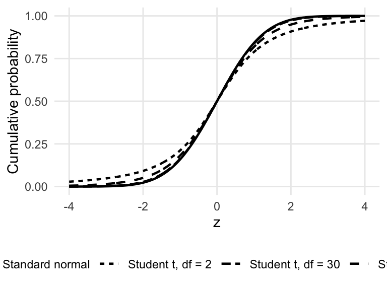
If \(T_{\nu}\) has a Student’s \(t\) distribution with \(\nu\) degrees of freedom, then \[T_{\nu}\overset{d}{\longrightarrow}\mathcal N(0,1) \qquad \text{as }\nu\to\infty.\]

The figure shows that the approximation improves as the degrees of freedom increase. Convergence in distribution does not mean that a particular draw from \(T_{\nu}\) becomes numerically close to a particular standard normal draw. It means that probabilities calculated under the two distributions become increasingly similar.

3.4.1 Random Vectors and Matrices

The definition extends to random vectors through their joint cumulative distribution functions. Let \(\mathbf X_n\) and \(\mathbf X\) be fixed-dimensional random vectors, and denote their joint cumulative distribution functions by \(F_{\mathbf X_n}\) and \(F_{\mathbf X}\).

Definition 3.13 (Convergence in Distribution for Random Vectors) The sequence \(\{\mathbf X_n\}\) converges in distribution to \(\mathbf X\) if \[\lim_{n\to\infty} F_{\mathbf X_n}(\mathbf z) = F_{\mathbf X}(\mathbf z)\] at every continuity point \(\mathbf z\) of \(F_{\mathbf X}\). We write \[\mathbf X_n\overset{d}{\longrightarrow}\mathbf X.\]

Convergence of each component separately is not, by itself, sufficient to establish convergence of the joint distribution because the dependence among the components must also converge. The Cramér–Wold device, introduced below, provides a convenient way to verify joint convergence.

For a sequence of random matrices of fixed dimension, convergence in distribution is defined by applying the vector definition to their vectorized forms. Thus, \[\mathbf A_n\overset{d}{\longrightarrow}\mathbf A\] means \[\operatorname{vec}(\mathbf A_n) \overset{d}{\longrightarrow} \operatorname{vec}(\mathbf A).\]

3.4.2 Relationship with Convergence in Probability

Convergence in probability is stronger than convergence in distribution. When two random variables are close with probability approaching one, their probability distributions must also become close.

Theorem 3.8 (Convergence in Probability Implies Convergence in Distribution) If \(X_n\overset{p}{\longrightarrow}X,\) then \(X_n\overset{d}{\longrightarrow}X.\)

The converse is not generally true. Two random variables may have increasingly similar distributions without becoming close to one another in probability. For example, let \(X\sim\mathcal N(0,1)\) and define \(X_n=-X\) for every \(n\). Then \(X_n\) and \(X\) have exactly the same distribution, so \[X_n\overset{d}{\longrightarrow}X.\]

Nevertheless, \[|X_n-X|=2|X|\] for every \(n\), and therefore \(X_n\) does not converge in probability to \(X\).

There is one important exception. When the limiting random variable is a constant, convergence in distribution and convergence in probability are equivalent.

Theorem 3.9 (Convergence to a Constant) Let \(c\) be a finite constant. Then \(X_n\overset{d}{\longrightarrow}c\) if and only if \(X_n\overset{p}{\longrightarrow}c.\)

The distribution concentrated at the single point \(c\) is called a degenerate distribution. Its cumulative distribution function has a jump at \(c\), which explains why the definition of convergence in distribution only requires convergence at continuity points of the limiting distribution.

Example 3.13 (A Nondegenerate Random Limit) Let \[Y_n = \left(2+\frac{1}{n}\right)X+3,\] where \(X\sim\mathcal N(1,2),\) with the second parameter denoting the variance. Define \(Y=2X+3.\) Then \[Y_n-Y = \frac{X}{n}.\]

Because \(X\) is finite with probability one, \[\frac{X}{n} \overset{a.s.}{\longrightarrow} 0,\] and therefore \[Y_n\overset{p}{\longrightarrow}Y.\]

By Theorem 3.8, \[Y_n\overset{d}{\longrightarrow}Y.\]

Finally, a linear transformation of a normal random variable is normal, so \[Y = 2X+3 \sim \mathcal N(5,8).\]

Thus, \[Y_n\overset{d}{\longrightarrow}\mathcal N(5,8).\]

This example also shows that a limiting distribution need not be degenerate. The random variables \(Y_n\) converge to the nonconstant random variable \(Y\).

3.4.3 Convergence in Distribution Does Not Imply Convergence of Moments

Convergence in distribution describes the behavior of cumulative distribution functions. It does not, without additional assumptions, guarantee convergence of means, variances, or higher-order moments.

Example 3.14 (Distributional Convergence without Moment Convergence) Define \[X_n = \begin{cases} n, & \text{with probability }1/n,\\ 0, & \text{with probability }1-1/n. \end{cases}\]

For any fixed \(\epsilon>0\) and all sufficiently large \(n\), \[\Pr\left(|X_n|>\epsilon\right) = \frac{1}{n} \longrightarrow 0.\]

Therefore, \(X_n\overset{p}{\longrightarrow}0\) and hence \(X_n\overset{d}{\longrightarrow}0.\) However, \(\mathbb E(X_n) = n\left(\frac{1}{n}\right) = 1\) for every \(n\), so \[\mathbb E(X_n) \not\longrightarrow 0 = \mathbb E(0).\]

Moreover, \[\mathbb E(X_n^2) = n^2\left(\frac{1}{n}\right) = n \longrightarrow \infty.\]

The example works because a very large value occurs with a probability that approaches zero. That rare event does not prevent convergence in probability or distribution, but it has a substantial effect on the moments. Additional conditions, such as uniform integrability, are needed to justify convergence of expectations from convergence in distribution.

3.4.4 Continuous Transformations and Slutsky’s Theorem

Two results are used repeatedly when deriving asymptotic distributions. The first allows us to apply continuous transformations to a convergent sequence. The second allows quantities that converge in probability to constants to be combined with quantities that converge in distribution.

Theorem 3.10 (Continuous Mapping Theorem for Convergence in Distribution) Suppose that \(\mathbf X_n\overset{d}{\longrightarrow}\mathbf X,\) and let \(g\) be continuous. Then \(g(\mathbf X_n) \overset{d}{\longrightarrow} g(\mathbf X).\)

Theorem 3.11 (Slutsky’s Theorem) Suppose that \(X_n\overset{d}{\longrightarrow}X\) and \(Y_n\overset{p}{\longrightarrow}c,\) where \(c\) is a finite constant. Then \[ \begin{aligned} X_n+Y_n &\overset{d}{\longrightarrow}X+c,\\ X_nY_n &\overset{d}{\longrightarrow}cX. \end{aligned} \]

If \(c\neq0\), then also \[\frac{X_n}{Y_n} \overset{d}{\longrightarrow} \frac{X}{c}.\]

More generally, \[\begin{pmatrix} X_n\\ Y_n \end{pmatrix} \overset{d}{\longrightarrow} \begin{pmatrix} X\\ c \end{pmatrix}.\]

The same argument applies to fixed-dimensional vectors and matrices.

Corollary 3.2 (Matrix Forms of Slutsky’s Theorem) Suppose that \(\mathbf x_n\overset{d}{\longrightarrow}\mathbf x\) and \(\mathbf A_n\overset{p}{\longrightarrow}\mathbf A,\) where \(\mathbf A\) is a constant matrix of fixed dimension. Then \[\mathbf A_n\mathbf x_n \overset{d}{\longrightarrow} \mathbf A\mathbf x.\]

If \(\mathbf A\) is nonsingular, then \[\mathbf A_n^{-1}\mathbf x_n \overset{d}{\longrightarrow} \mathbf A^{-1}\mathbf x\] and \[\mathbf x_n^{\top} \mathbf A_n^{-1} \mathbf x_n \overset{d}{\longrightarrow} \mathbf x^{\top} \mathbf A^{-1} \mathbf x.\]

The nonsingularity of \(\mathbf A\) ensures, by continuity of matrix inversion, that \(\mathbf A_n\) is nonsingular with probability approaching one and that \(\mathbf A_n^{-1}\overset{p}{\longrightarrow}\mathbf A^{-1}\). If \(\mathbf x\sim\mathcal N(\mathbf 0,\boldsymbol\Sigma)\), then \(\mathbf A\mathbf x\sim\mathcal N\left(\mathbf 0,\mathbf A\boldsymbol\Sigma\mathbf A^{\top}\right)\).

Example 3.15 (A Matrix Transformation of a Limiting Normal Vector) Suppose that \[\mathbf A_n \overset{p}{\longrightarrow} \mathbf A = \begin{pmatrix} 3&2\\ 2&4 \end{pmatrix}\] and \[\mathbf y_n \overset{d}{\longrightarrow} \mathbf y \sim \mathcal N(\mathbf 0,\mathbf I_2).\]

By the matrix form of Slutsky’s theorem, \[\mathbf A_n\mathbf y_n \overset{d}{\longrightarrow} \mathbf A\mathbf y.\]

Because \(\mathbf y\) has covariance matrix \(\mathbf I_2\), \[\begin{aligned} \operatorname{Var}(\mathbf A\mathbf y) &= \mathbf A\mathbf I_2\mathbf A^{\top}\\ &= \mathbf A\mathbf A^{\top}\\ &= \begin{pmatrix} 13&14\\ 14&20 \end{pmatrix}. \end{aligned}\]

Therefore, \[\mathbf A_n\mathbf y_n \overset{d}{\longrightarrow} \mathcal N \left( \mathbf 0, \begin{pmatrix} 13&14\\ 14&20 \end{pmatrix} \right).\]

Moreover, \[\mathbf A^{-1} = \begin{pmatrix} 0.5&-0.25\\ -0.25&0.375 \end{pmatrix}.\]

Since \(\mathbf A^{-1}\) is symmetric, \[\begin{aligned} \operatorname{Var}(\mathbf A^{-1}\mathbf y) &= \mathbf A^{-1} (\mathbf A^{-1})^{\top}\\ &= \begin{pmatrix} 0.3125&-0.21875\\ -0.21875&0.203125 \end{pmatrix}. \end{aligned}\]

Thus, \[\mathbf A_n^{-1}\mathbf y_n \overset{d}{\longrightarrow} \mathcal N \left( \mathbf 0, \begin{pmatrix} 0.3125&-0.21875\\ -0.21875&0.203125 \end{pmatrix} \right).\]

A useful scalar application of the continuous mapping theorem is obtained by squaring a Student’s \(t\) random variable. If \[T_{\nu}\overset{d}{\longrightarrow}Z, \qquad Z\sim\mathcal N(0,1),\] then \[T_{\nu}^2 \overset{d}{\longrightarrow} Z^2 \sim \chi_1^2.\]

Because \(T_{\nu}^2\) has an \(F_{1,\nu}\) distribution, \[F_{1,\nu} \overset{d}{\longrightarrow} \chi_1^2.\]

3.4.5 An Estimator Can Be Consistent without Having Finite Moments

The following example combines consistency, limiting distributions, and the failure of finite-sample moments.

Example 3.16 (The Inverse of a Normal Sample Mean) Let \(Y_1,\ldots,Y_n\) be independently and identically distributed as \(Y_i\sim\mathcal N(\mu,\sigma^2)\), \(\mu\neq0.\) The sample mean satisfies \[\overline Y_n \overset{p}{\longrightarrow} \mu. \]

Since the function \(g(y)=1/y\) is continuous at \(\mu\neq0\), the continuous mapping theorem gives \[\overline Y_n^{-1} \overset{p}{\longrightarrow} \mu^{-1}.\]

Thus, \(\overline Y_n^{-1}\) is a consistent estimator of \(\mu^{-1}\). For every \(n\), \[\sqrt n \left( \overline Y_n- \mu \right) \sim \mathcal N(0,\sigma^2).\]

Using the identity \[\frac{1}{\overline Y_n}-\frac{1}{\mu} = -\frac{\overline Y_n-\mu} {\mu\overline Y_n},\] we obtain \[\sqrt n \left( \overline Y_n^{-1}-\mu^{-1} \right) = -\frac{1}{\mu\overline Y_n} \sqrt n \left( \overline Y_n- \mu \right).\]

Consistency of \(\overline Y_n\) implies \[-\frac{1}{\mu\overline Y_n} \overset{p}{\longrightarrow} -\frac{1}{\mu^2}.\]

Slutsky’s theorem therefore yields \[\sqrt n \left( \overline Y_n^{-1}-\mu^{-1} \right) \overset{d}{\longrightarrow} \mathcal N \left( 0, \frac{\sigma^2}{\mu^4} \right).\]

Nevertheless, \(\overline Y_n\) has a normal density that is strictly positive in a neighborhood of zero. Consequently, the integral defining \[\mathbb E\left( \left| \overline Y_n^{-1} \right| \right)\] diverges because \(1/|y|\) is not integrable around zero. Hence \(\overline Y_n^{-1}\) does not possess a finite first absolute moment, and its ordinary expectation and variance are not well defined.

This example demonstrates that consistency and asymptotic normality do not require finite-sample moments of the estimator itself. It also reinforces the point that the moments of a limiting distribution need not equal the limits of finite-sample moments.

3.4.6 Asymptotic Equivalence

Two sequences that differ by an amount converging in probability to zero have the same limiting distribution.

Lemma 3.1 (Asymptotic Equivalence) Suppose that \(Y_n-X_n \overset{p}{\longrightarrow} 0\) and \(X_n\overset{d}{\longrightarrow}X.\) Then \[Y_n\overset{d}{\longrightarrow}X.\]

Proof. Write \(Y_n =X_n+(Y_n-X_n)\). By assumption, \(X_n\overset{d}{\longrightarrow}X\) and \(Y_n-X_n\overset{p}{\longrightarrow}0\). Applying Slutsky’s theorem (Theorem 3.11) to the sum gives \(Y_n\overset{d}{\longrightarrow}X+0=X\).

The lemma is especially useful when the distribution of \(Y_n\) is difficult to analyze directly. It is enough to find a simpler sequence \(X_n\) with a known limiting distribution and show that the difference between the two sequences is asymptotically negligible.

3.4.7 The Cramér–Wold Device

For a random vector, convergence of each marginal component is not sufficient to establish convergence of the joint distribution. The Cramér–Wold device instead considers every linear combination of the vector’s components.

Theorem 3.12 (Cramér–Wold Device) Let \(\mathbf X_n\) and \(\mathbf X\) be \(k\times1\) random vectors, where \(k\) is fixed. Then \[\mathbf X_n\overset{d}{\longrightarrow}\mathbf X\] if and only if \[\mathbf c^{\top}\mathbf X_n \overset{d}{\longrightarrow} \mathbf c^{\top}\mathbf X\] for every fixed vector \(\mathbf c\in\mathbb R^k\).

The Cramér–Wold device is particularly valuable for proving multivariate central limit theorems. Instead of deriving the joint limiting distribution directly, one can prove a scalar central limit theorem for every linear combination \(\mathbf c^{\top}\mathbf X_n\).

3.5 Central Limit Theorems

The laws of large numbers explain why sample averages and many econometric estimators converge to fixed population quantities. This is enough to establish consistency, but it is not enough for statistical inference. To construct confidence intervals and hypothesis tests, we also need to know how the sampling distribution of an estimator behaves around its probability limit.

Suppose that an estimator satisfies \(\widehat{\boldsymbol\theta}_n\overset{p}{\longrightarrow}\boldsymbol\theta_0.\) Convergence in probability implies convergence in distribution, so \(\widehat{\boldsymbol\theta}_n\overset{d}{\longrightarrow}\boldsymbol\theta_0.\) This limiting distribution is degenerate: all of its probability mass is concentrated at the single point \(\boldsymbol\theta_0\). Although this result confirms consistency, it does not describe the uncertainty that remains in a large but finite sample.

The useful limiting distribution is usually obtained by centering the estimator at the true parameter and rescaling the estimation error. In many applications, the appropriate normalization is \(\sqrt n\): \[\sqrt n \left( \widehat{\boldsymbol\theta}_n- \boldsymbol\theta_0 \right) \overset{d}{\longrightarrow} \mathbf Z,\] where \(\mathbf Z\) has a proper, nondegenerate distribution. When this occurs, the estimation error is typically of order \(1/\sqrt n\), and the estimator is said to be root-\(n\) consistent. Central limit theorems often establish that \(\mathbf Z\) has a normal distribution.

3.5.1 Why the Sample Mean Must Be Rescaled

Consider an independent and identically distributed sample \(X_1,\ldots,X_n\) with \(\mathbb E(X_i)=\mu\), and \(\operatorname{Var}(X_i)=\sigma^2\). The sample mean satisfies \(\mathbb E(\overline X_n)=\mu\), and \(\operatorname{Var}(\overline X_n)=\frac{\sigma^2}{n}\). Therefore, the distribution of \(\overline X_n\) becomes increasingly concentrated around \(\mu\). In fact, \(\overline X_n\overset{p}{\longrightarrow}\mu\).

To prevent the variance from collapsing to zero, define \[Z_n = \sqrt n(\overline X_n-\mu).\]

Then \[\mathbb E(Z_n)=0\] and \[\operatorname{Var}(Z_n) = n\operatorname{Var}(\overline X_n) = \sigma^2.\]

The multiplication by \(\sqrt n\) exactly offsets the rate at which the variance of the sample mean decreases. A central limit theorem determines the limiting shape of the distribution that remains after this normalization.

Figure 3.7 illustrates the distinction between the law of large numbers and the central limit theorem. The underlying observations are exponentially distributed and therefore strongly right-skewed. For each sample size, the figure reports the repeated-sampling distribution of the standardized sample mean \[\sqrt n(\overline X_n-1),\] where an exponential random variable with rate one has mean and variance equal to one.

Figure 3.7: Standardized sample means from an exponential population

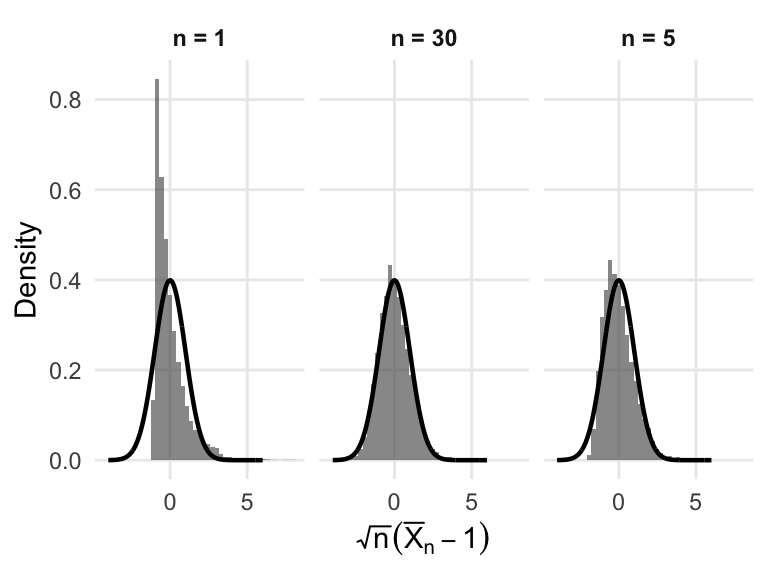
When \(n=1\), the standardized mean retains the pronounced asymmetry of the exponential population. As \(n\) increases, its distribution becomes more symmetric and increasingly resembles the standard normal density. The law of large numbers explains why \(\overline X_n\) approaches one; the central limit theorem explains the shape of the remaining sampling variation after the error is multiplied by \(\sqrt n\).

3.5.2 The Univariate Lindeberg–Lévy Central Limit Theorem

Theorem 3.13 (Univariate Lindeberg–Lévy Central Limit Theorem) Let \(X_1,X_2,\ldots\) be independent and identically distributed random variables such that \(\mathbb E(X_i)=\mu\) and \(0<\operatorname{Var}(X_i)=\sigma^2<\infty.\) Then \[\frac{\sqrt n(\overline X_n-\mu)}{\sigma} = \frac{1}{\sigma\sqrt n} \sum_{i=1}^{n}(X_i-\mu) \overset{d}{\longrightarrow} \mathcal N(0,1).\]

Equivalently, \[\sqrt n(\overline X_n-\mu) \overset{d}{\longrightarrow} \mathcal N(0,\sigma^2).\]

The theorem does not require the population itself to be normally distributed. It states that the standardized sample mean becomes approximately normal when the sample is sufficiently large, provided the observations are i.i.d. and have a finite, strictly positive variance.

For a large but finite \(n\), the result motivates the approximation \[\overline X_n \mathrel{\dot\sim} \mathcal N\left( \mu, \frac{\sigma^2}{n} \right),\] where \(\mathrel{\dot\sim}\) indicates an approximation rather than an exact distributional equality.

ImportantWhat the central limit theorem does and does not say

The theorem does not say that a large population is approximately normal. It concerns the repeated-sampling distribution of a normalized sample mean. It also does not imply that \(\overline X_n\) converges to a nondegenerate normal distribution. Without normalization, \[\overline X_n\overset{p}{\longrightarrow}\mu,\] so its limiting distribution is a point mass at \(\mu\). The normal approximation \[\mathcal N\left(\mu,\frac{\sigma^2}{n}\right)\] is an \(n\)-dependent approximation for large finite samples; its variance also converges to zero.

3.5.3 The Multivariate Lindeberg–Lévy Central Limit Theorem

Many econometric estimators depend on averages of random vectors rather than scalar random variables. Let \[\mathbf X_i = \begin{pmatrix} X_{i1}\\ X_{i2}\\ \vdots\\ X_{iK} \end{pmatrix}\] have mean vector \[\boldsymbol\mu = \mathbb E(\mathbf X_i)\] and covariance matrix \[\mathbf Q = \operatorname{Var}(\mathbf X_i).\]

The vector sample mean is \[\overline{\mathbf X}_n = \frac{1}{n}\sum_{i=1}^{n}\mathbf X_i.\]

Theorem 3.14 (Multivariate Lindeberg–Lévy Central Limit Theorem) Let \(\mathbf X_1,\mathbf X_2,\ldots\) be independent and identically distributed random vectors of fixed dimension \(K\). Suppose that \(\mathbb E(\mathbf X_i)=\boldsymbol\mu\) and that \(\mathbf Q=\operatorname{Var}(\mathbf X_i)\) is finite. Then \[\sqrt n \left( \overline{\mathbf X}_n- \boldsymbol\mu \right) \overset{d}{\longrightarrow} \mathcal N(\mathbf 0,\mathbf Q).\]

The limiting normal distribution may be singular when \(\mathbf Q\) is singular. If \(\mathbf Q\) is positive definite, the limiting distribution is nondegenerate.

Proof. Let \(\mathbf c\in\mathbb R^K\) be an arbitrary fixed vector. Consider the scalar projection \[U_i = \mathbf c^{\top}\mathbf X_i.\]

Because the \(\mathbf X_i\) are i.i.d., the \(U_i\) are also i.i.d (see Proposition 3.5). Their mean is \[\mathbb E(U_i) = \mathbf c^{\top}\boldsymbol\mu,\] and their variance is \[\begin{aligned} \operatorname{Var}(U_i) &= \operatorname{Var}\left( \mathbf c^{\top}\mathbf X_i \right)\\ &= \mathbf c^{\top}\mathbf Q\mathbf c. \end{aligned}\]

If \(\mathbf c^{\top}\mathbf Q\mathbf c>0\), the univariate central limit theorem gives \[\sqrt n \left( \overline U_n- \mathbf c^{\top}\boldsymbol\mu \right) \overset{d}{\longrightarrow} \mathcal N\left( 0, \mathbf c^{\top}\mathbf Q\mathbf c \right).\]

Since \[\overline U_n = \mathbf c^{\top}\overline{\mathbf X}_n,\] we have \[\mathbf c^{\top} \sqrt n \left( \overline{\mathbf X}_n- \boldsymbol\mu \right) \overset{d}{\longrightarrow} \mathcal N\left( 0, \mathbf c^{\top}\mathbf Q\mathbf c \right).\]

If \(\mathbf c^{\top}\mathbf Q\mathbf c=0\), then \[\operatorname{Var}\left( \mathbf c^{\top}\mathbf X_i \right)=0,\] so \[\mathbf c^{\top}\mathbf X_i = \mathbf c^{\top}\boldsymbol\mu\] almost surely. The corresponding normalized projection is therefore identically zero, which is the degenerate normal distribution with variance zero.

Thus, for every fixed \(\mathbf c\in\mathbb R^K\), \[\mathbf c^{\top} \sqrt n \left( \overline{\mathbf X}_n- \boldsymbol\mu \right) \overset{d}{\longrightarrow} \mathbf c^{\top}\mathbf Z,\] where \[\mathbf Z\sim\mathcal N(\mathbf 0,\mathbf Q).\]

The Cramér–Wold device in Theorem 3.12 then implies \[\sqrt n \left( \overline{\mathbf X}_n- \boldsymbol\mu \right) \overset{d}{\longrightarrow} \mathcal N(\mathbf 0,\mathbf Q).\]

3.5.4 Independent but Non-Identically Distributed Observations

The i.i.d. assumption is often too restrictive. In cross-sectional data, for example, observations may have different variances even when they are independent. The Lindeberg–Feller theorem allows the distributions to differ across observations, but it requires a condition ensuring that no small number of extreme observations dominates the variance of the normalized sum.

Let \(X_1,X_2,\ldots\) be independent random variables with \[\mathbb E(X_i)=\mu_i\] and \[\operatorname{Var}(X_i)=\sigma_i^2.\]

Define \[s_n^2 = \sum_{i=1}^{n}\sigma_i^2,\] and suppose that \(s_n^2>0\).

Theorem 3.15 (Univariate Lindeberg–Feller Central Limit Theorem) Suppose that \(X_1,X_2,\ldots\) are independent, that \(s_n^2\to\infty\), and that for every \(\epsilon>0\), \[\frac{1}{s_n^2} \sum_{i=1}^{n} \mathbb E\left[ (X_i-\mu_i)^2 \mathbf 1\left\{ |X_i-\mu_i|>\epsilon s_n \right\} \right] \longrightarrow0. \tag{3.7}\]

Then \[\frac{ \sum_{i=1}^{n}(X_i-\mu_i) }{s_n} \overset{d}{\longrightarrow} \mathcal N(0,1).\]

The condition in Equation 3.7 is called the Lindeberg condition (see also Theorem 5.6 in White 2014). The numerator inside the expectation records the contribution to variance from observations whose centered magnitude exceeds a fixed fraction of the standard deviation of the complete sum. The condition requires the aggregate contribution of such unusually large observations to become negligible.

To express the result in terms of sample averages, define \[\overline\mu_n = \frac{1}{n}\sum_{i=1}^{n}\mu_i\] and \[\overline\sigma_n^2 = \frac{1}{n}\sum_{i=1}^{n}\sigma_i^2.\]

Since \[s_n = \sqrt n\,\overline\sigma_n,\] the conclusion can be written as \[\frac{ \sqrt n(\overline X_n-\overline\mu_n) }{\overline\sigma_n} \overset{d}{\longrightarrow} \mathcal N(0,1).\]

NoteA no-dominant-observation condition is not enough by itself

The requirement \[\max_{1\leq i\leq n} \frac{\sigma_i^2}{s_n^2} \longrightarrow0\] expresses the useful intuition that no individual observation should account for a nonnegligible share of the total variance. This condition is implied by the Lindeberg condition, but it is not generally sufficient on its own to establish asymptotic normality. The behavior of the tails must also be controlled.

3.5.5 The Lyapunov Condition

The Lindeberg condition is general, but its indicator function can make it difficult to verify directly. A stronger but often simpler sufficient condition is based on moments of order slightly greater than two (compare with Theorem 5.10 in White 2014).

Theorem 3.16 (Lyapunov Central Limit Theorem) Let \(X_1,X_2,\ldots\) be independent random variables with means \(\mu_i\) and finite, positive variances \(\sigma_i^2\). Define \[s_n^2 = \sum_{i=1}^{n}\sigma_i^2.\]

Suppose that \(s_n^2\to\infty\) and that, for some \(\delta>0\), \[\frac{1}{s_n^{2+\delta}} \sum_{i=1}^{n} \mathbb E\left( |X_i-\mu_i|^{2+\delta} \right) \longrightarrow0. \tag{3.8}\]

Then \[\frac{ \sum_{i=1}^{n}(X_i-\mu_i) }{s_n} \overset{d}{\longrightarrow} \mathcal N(0,1).\]

Proof. Fix an arbitrary \(\epsilon>0\). On the event \[|X_i-\mu_i|>\epsilon s_n,\] we have \[|X_i-\mu_i|^{\delta} > \epsilon^{\delta}s_n^{\delta}.\]

Therefore, \[\mathbf 1\left\{ |X_i-\mu_i|>\epsilon s_n \right\} \leq \frac{|X_i-\mu_i|^{\delta}} {\epsilon^{\delta}s_n^{\delta}}.\]

Multiplying both sides by \((X_i-\mu_i)^2\) gives \[ \begin{aligned} (X_i-\mu_i)^2 \mathbf 1\left\{ |X_i-\mu_i|>\epsilon s_n \right\} \leq \frac{|X_i-\mu_i|^{2+\delta}} {\epsilon^{\delta}s_n^{\delta}}. \end{aligned} \]

Taking expectations, summing over \(i\), and dividing by \(s_n^2\) yields \[\begin{aligned} &\frac{1}{s_n^2} \sum_{i=1}^{n} \mathbb E\left[ (X_i-\mu_i)^2 \mathbf 1\left\{ |X_i-\mu_i|>\epsilon s_n \right\} \right] \leq \frac{1}{\epsilon^{\delta}} \frac{1}{s_n^{2+\delta}} \sum_{i=1}^{n} \mathbb E\left( |X_i-\mu_i|^{2+\delta} \right). \end{aligned}\]

By Equation 3.8, the expression on the right converges to zero. Hence the Lindeberg condition in Equation 3.7 holds. The conclusion then follows from the Lindeberg–Feller central limit theorem in Theorem 3.15.

The Lyapunov condition requires more than the existence of moments of order \(2+\delta\). It requires their sum to be small relative to the total variance raised to the power \(1+\delta/2\). This distinction is important: finite higher moments alone do not guarantee a central limit theorem for a non-identically distributed sequence.

3.5.6 A Multivariate Lindeberg–Feller Theorem

The non-identically distributed result also extends to fixed-dimensional random vectors.

Theorem 3.17 (Multivariate Lindeberg–Feller Central Limit Theorem) Let \(\mathbf X_1,\mathbf X_2,\ldots\) be independent random vectors in \(\mathbb R^K\), with \[\mathbb E(\mathbf X_i)=\boldsymbol\mu_i.\]

Define \[\overline{\boldsymbol\mu}_n = \frac{1}{n}\sum_{i=1}^{n}\boldsymbol\mu_i\] and \[\mathbf Q_n = \frac{1}{n} \sum_{i=1}^{n} \operatorname{Var}(\mathbf X_i).\]

Suppose that \[\mathbf Q_n\longrightarrow\mathbf Q,\] where \(\mathbf Q\) is finite, and that for every \(\epsilon>0\), \[\frac{1}{n} \sum_{i=1}^{n} \mathbb E\left[ \left\| \mathbf X_i-\boldsymbol\mu_i \right\|^2 \mathbf 1\left\{ \left\| \mathbf X_i-\boldsymbol\mu_i \right\|>\epsilon\sqrt n \right\} \right] \longrightarrow0. \tag{3.9}\]

Then \[\sqrt n \left( \overline{\mathbf X}_n- \overline{\boldsymbol\mu}_n \right) \overset{d}{\longrightarrow} \mathcal N(\mathbf 0,\mathbf Q).\]

Proof. Let \(\mathbf c\in\mathbb R^K\) be fixed. If \(\mathbf c=\mathbf 0\), the desired convergence for the projection is immediate. Suppose therefore that \(\mathbf c\neq\mathbf 0\) and define \[U_i = \mathbf c^{\top} \left( \mathbf X_i-\boldsymbol\mu_i \right).\]

The variables \(U_i\) are independent and have mean zero. Their average variance satisfies \[\begin{aligned} \frac{1}{n} \sum_{i=1}^{n}\operatorname{Var}(U_i) &= \frac{1}{n} \sum_{i=1}^{n} \mathbf c^{\top} \operatorname{Var}(\mathbf X_i) \mathbf c\\ &= \mathbf c^{\top}\mathbf Q_n\mathbf c\\ &\longrightarrow \mathbf c^{\top}\mathbf Q\mathbf c. \end{aligned}\]

Assume first that \[\mathbf c^{\top}\mathbf Q\mathbf c>0.\]

Let \[s_{n,\mathbf c}^2 = \sum_{i=1}^{n}\operatorname{Var}(U_i) = n\mathbf c^{\top}\mathbf Q_n\mathbf c.\]

Because \[\mathbf c^{\top}\mathbf Q_n\mathbf c \longrightarrow \mathbf c^{\top}\mathbf Q\mathbf c>0,\] there exist a constant \(a_{\mathbf c}>0\) and an integer \(N\) such that \[s_{n,\mathbf c} \geq a_{\mathbf c}\sqrt n\] for every \(n\geq N\).

By the Cauchy–Schwarz inequality, \[|U_i| \leq \|\mathbf c\| \left\| \mathbf X_i-\boldsymbol\mu_i \right\|.\]

Hence the event \[|U_i|>\epsilon s_{n,\mathbf c}\] implies \[\left\| \mathbf X_i-\boldsymbol\mu_i \right\| > \frac{\epsilon a_{\mathbf c}}{\|\mathbf c\|} \sqrt n.\]

Also, \[U_i^2 \leq \|\mathbf c\|^2 \left\| \mathbf X_i-\boldsymbol\mu_i \right\|^2.\]

Therefore, \[\begin{aligned} &\frac{1}{s_{n,\mathbf c}^2} \sum_{i=1}^{n} \mathbb E\left[ U_i^2 \mathbf 1\left\{ |U_i|>\epsilon s_{n,\mathbf c} \right\} \right]\\ &\qquad\leq \frac{\|\mathbf c\|^2} {a_{\mathbf c}^2n} \sum_{i=1}^{n} \mathbb E\left[ \left\| \mathbf X_i-\boldsymbol\mu_i \right\|^2 \mathbf 1\left\{ \left\| \mathbf X_i-\boldsymbol\mu_i \right\| > \frac{\epsilon a_{\mathbf c}}{\|\mathbf c\|} \sqrt n \right\} \right]. \end{aligned}\]

The right-hand side converges to zero by Equation 3.9. Thus the scalar Lindeberg condition holds for the sequence \(\{U_i\}\), and \[\frac{\sum_{i=1}^{n}U_i}{s_{n,\mathbf c}} \overset{d}{\longrightarrow} \mathcal N(0,1).\]

Since \[\frac{s_{n,\mathbf c}}{\sqrt n} = \left( \mathbf c^{\top}\mathbf Q_n\mathbf c \right)^{1/2} \longrightarrow \left( \mathbf c^{\top}\mathbf Q\mathbf c \right)^{1/2},\]

Slutsky’s theorem gives \[\frac{1}{\sqrt n} \sum_{i=1}^{n}U_i \overset{d}{\longrightarrow} \mathcal N\left( 0, \mathbf c^{\top}\mathbf Q\mathbf c \right).\]

If instead \[\mathbf c^{\top}\mathbf Q\mathbf c=0,\] then \[\operatorname{Var}\left( \frac{1}{\sqrt n}\sum_{i=1}^{n}U_i \right) = \mathbf c^{\top}\mathbf Q_n\mathbf c \longrightarrow0.\]

Chebyshev’s inequality implies \[\frac{1}{\sqrt n}\sum_{i=1}^{n}U_i \overset{p}{\longrightarrow}0.\]

Thus, for every \(\mathbf c\in\mathbb R^K\), \[\mathbf c^{\top} \sqrt n \left( \overline{\mathbf X}_n- \overline{\boldsymbol\mu}_n \right) \overset{d}{\longrightarrow} \mathcal N\left( 0, \mathbf c^{\top}\mathbf Q\mathbf c \right).\]

The Cramér–Wold device in Theorem 3.12 completes the proof.

3.5.7 Application: Asymptotic Normality of OLS

The multivariate central limit theorem becomes useful in econometrics when an estimator can be written as a sample average, or as a smooth transformation of sample averages. Ordinary least squares provides the basic example.

Consider the linear regression model \[y_i = \mathbf x_i^{\top}\boldsymbol\beta_0 + \varepsilon_i, \qquad i=1,\ldots,n,\] where \(\mathbf x_i\) is a \(K\times1\) vector. The OLS estimator is \[\widehat{\boldsymbol\beta}_n = \left( \sum_{i=1}^{n}\mathbf x_i\mathbf x_i^{\top} \right)^{-1} \sum_{i=1}^{n}\mathbf x_i y_i.\]

Theorem 3.18 (Asymptotic Normality of OLS under Random Sampling) Suppose that \(\{(y_i,\mathbf x_i)\}_{i=1}^{n}\) is an i.i.d. random sample and that \[y_i = \mathbf x_i^{\top}\boldsymbol\beta_0 + \varepsilon_i.\]

Assume that \[\mathbb E(\mathbf x_i\varepsilon_i)=\mathbf 0,\] that \[\mathbf Q = \mathbb E(\mathbf x_i\mathbf x_i^{\top})\] is finite and positive definite, and that \[\boldsymbol\Omega = \mathbb E\left( \varepsilon_i^2 \mathbf x_i\mathbf x_i^{\top} \right)\] is finite. Then \[\sqrt n \left( \widehat{\boldsymbol\beta}_n- \boldsymbol\beta_0 \right) \overset{d}{\longrightarrow} \mathcal N\left( \mathbf 0, \mathbf Q^{-1} \boldsymbol\Omega \mathbf Q^{-1} \right).\]

Proof. Substituting \[y_i = \mathbf x_i^{\top}\boldsymbol\beta_0 + \varepsilon_i\] into the OLS formula gives \[\begin{aligned} \widehat{\boldsymbol\beta}_n &= \left( \sum_{i=1}^{n}\mathbf x_i\mathbf x_i^{\top} \right)^{-1} \sum_{i=1}^{n} \mathbf x_i \left( \mathbf x_i^{\top}\boldsymbol\beta_0 + \varepsilon_i \right)\\ &= \left( \sum_{i=1}^{n}\mathbf x_i\mathbf x_i^{\top} \right)^{-1} \left( \sum_{i=1}^{n} \mathbf x_i\mathbf x_i^{\top} \right) \boldsymbol\beta_0 + \left( \sum_{i=1}^{n}\mathbf x_i\mathbf x_i^{\top} \right)^{-1} \sum_{i=1}^{n}\mathbf x_i\varepsilon_i\\ &= \boldsymbol\beta_0 + \left( \sum_{i=1}^{n}\mathbf x_i\mathbf x_i^{\top} \right)^{-1} \sum_{i=1}^{n}\mathbf x_i\varepsilon_i. \end{aligned}\]

Therefore, \[\widehat{\boldsymbol\beta}_n- \boldsymbol\beta_0 = \left( \sum_{i=1}^{n}\mathbf x_i\mathbf x_i^{\top} \right)^{-1} \sum_{i=1}^{n}\mathbf x_i\varepsilon_i.\]

Multiplying by \(\sqrt n\) and introducing the appropriate normalizations gives \[\sqrt n \left( \widehat{\boldsymbol\beta}_n- \boldsymbol\beta_0 \right) = \left( \frac{1}{n} \sum_{i=1}^{n} \mathbf x_i\mathbf x_i^{\top} \right)^{-1} \left( \frac{1}{\sqrt n} \sum_{i=1}^{n} \mathbf x_i\varepsilon_i \right). \tag{3.10}\]

By the law of large numbers, \[\frac{1}{n} \sum_{i=1}^{n} \mathbf x_i\mathbf x_i^{\top} \overset{p}{\longrightarrow} \mathbb E(\mathbf x_i\mathbf x_i^{\top}) = \mathbf Q.\]

Because \(\mathbf Q\) is positive definite, it is nonsingular. The continuous mapping theorem therefore implies \[\left( \frac{1}{n} \sum_{i=1}^{n} \mathbf x_i\mathbf x_i^{\top} \right)^{-1} \overset{p}{\longrightarrow} \mathbf Q^{-1}.\]

Next, define \[\mathbf z_i = \mathbf x_i\varepsilon_i.\]

The orthogonality condition gives \[\mathbb E(\mathbf z_i) = \mathbb E(\mathbf x_i\varepsilon_i) = \mathbf 0.\]

Its covariance matrix is \[\begin{aligned} \operatorname{Var}(\mathbf z_i) &= \mathbb E(\mathbf z_i\mathbf z_i^{\top})\\ &= \mathbb E\left( \varepsilon_i^2 \mathbf x_i\mathbf x_i^{\top} \right)\\ &= \boldsymbol\Omega. \end{aligned}\]

The multivariate central limit theorem in Theorem 3.14 therefore gives \[\frac{1}{\sqrt n} \sum_{i=1}^{n} \mathbf x_i\varepsilon_i \overset{d}{\longrightarrow} \mathcal N(\mathbf 0,\boldsymbol\Omega).\]

Combining these two limits in Equation 3.10 and applying Slutsky’s theorem yields \[\sqrt n \left( \widehat{\boldsymbol\beta}_n- \boldsymbol\beta_0 \right) \overset{d}{\longrightarrow} \mathcal N\left( \mathbf 0, \mathbf Q^{-1} \boldsymbol\Omega (\mathbf Q^{-1})^{\top} \right).\]

Since \(\mathbf Q\) is symmetric, \(\mathbf Q^{-1}\) is also symmetric, so \[(\mathbf Q^{-1})^{\top} = \mathbf Q^{-1}.\]

Hence \[\sqrt n \left( \widehat{\boldsymbol\beta}_n- \boldsymbol\beta_0 \right) \overset{d}{\longrightarrow} \mathcal N\left( \mathbf 0, \mathbf Q^{-1} \boldsymbol\Omega \mathbf Q^{-1} \right).\]

Under conditional homoskedasticity, \[\mathbb E(\varepsilon_i^2\mid\mathbf x_i) = \sigma^2,\] we obtain \[\begin{aligned} \boldsymbol\Omega &= \mathbb E\left[ \mathbb E(\varepsilon_i^2\mid\mathbf x_i) \mathbf x_i\mathbf x_i^{\top} \right]\\ &= \sigma^2 \mathbb E(\mathbf x_i\mathbf x_i^{\top})\\ &= \sigma^2\mathbf Q. \end{aligned}\]

The asymptotic covariance matrix then simplifies to \[\mathbf Q^{-1} \boldsymbol\Omega \mathbf Q^{-1} = \sigma^2\mathbf Q^{-1}.\]

This example displays the standard structure of many asymptotic-normality arguments in econometrics:

1. rewrite the normalized estimation error as a product of sample averages;
2. apply a law of large numbers to the matrix term;
3. apply a central limit theorem to the centered score or moment term; and
4. combine the limits using Slutsky’s theorem.

3.5.8 Asymptotic Covariance and Studentization

Definition 3.14 (Asymptotic Covariance Matrix) Suppose that \[\sqrt n \left( \widehat{\boldsymbol\theta}_n- \boldsymbol\theta_0 \right) \overset{d}{\longrightarrow} \mathcal N(\mathbf 0,\mathbf V),\] where \(\mathbf V\) is finite. Then \(\mathbf V\) is the asymptotic covariance matrix of the normalized estimator. Equivalently, for large \(n\), \[\widehat{\boldsymbol\theta}_n \mathrel{\dot\sim} \mathcal N\left( \boldsymbol\theta_0, \frac{\mathbf V}{n} \right).\]

Under this convention, \(\mathbf V/n\) is the asymptotic covariance approximation for the unnormalized estimator \(\widehat{\boldsymbol\theta}_n\).

The distinction between \(\mathbf V\) and \(\mathbf V/n\) should always be made explicit. Some texts use “asymptotic variance” for \(\mathbf V\), while others use it for \(\mathbf V/n\). Stating the normalization avoids ambiguity.

A feasible statistic replaces the unknown matrix \(\mathbf V\) with a consistent estimator.

Theorem 3.19 (Studentized Asymptotic Normality) Suppose that \[\sqrt n \left( \widehat{\boldsymbol\theta}_n- \boldsymbol\theta_0 \right) \overset{d}{\longrightarrow} \mathcal N(\mathbf 0,\mathbf V),\] where \(\mathbf V\) is positive definite, and suppose that \[\widehat{\mathbf V}_n \overset{p}{\longrightarrow} \mathbf V.\]

Then \[\widehat{\mathbf V}_n^{-1/2} \sqrt n \left( \widehat{\boldsymbol\theta}_n- \boldsymbol\theta_0 \right) \overset{d}{\longrightarrow} \mathcal N(\mathbf 0,\mathbf I).\]

Proof. Because \(\mathbf V\) is positive definite, the function \(\mathbf A\mapsto\mathbf A^{-1/2}\) is continuous on a neighborhood of \(\mathbf V\) within the set of positive definite matrices. The continuous mapping theorem therefore gives \(\widehat{\mathbf V}_n^{-1/2} \overset{p}{\longrightarrow} \mathbf V^{-1/2}.\)

Slutsky’s theorem then implies \[\begin{aligned} &\widehat{\mathbf V}_n^{-1/2} \sqrt n \left( \widehat{\boldsymbol\theta}_n- \boldsymbol\theta_0 \right) \overset{d}{\longrightarrow} \mathbf V^{-1/2}\mathbf Z, \end{aligned}\] where \(\mathbf Z\sim\mathcal N(\mathbf 0,\mathbf V).\)

A linear transformation of a multivariate normal vector is normal, and \[\operatorname{Var} \left( \mathbf V^{-1/2}\mathbf Z \right) = \mathbf V^{-1/2} \mathbf V \mathbf V^{-1/2} = \mathbf I.\]

Hence \[\mathbf V^{-1/2}\mathbf Z \sim \mathcal N(\mathbf 0,\mathbf I),\] which proves the result.

For an individual component \(j\), the theorem implies \[\frac{ \widehat\theta_{nj}-\theta_{0j} }{ \sqrt{\widehat V_{n,jj}/n} } \overset{d}{\longrightarrow} \mathcal N(0,1).\]

This standardized statistic is the basis for asymptotic confidence intervals and large-sample tests. The central limit theorem therefore supplies the limiting distribution, while consistent covariance estimation makes the result operational.

3.6 Orders in Probability

The deterministic order symbols \(O(\cdot)\) and \(o(\cdot)\) describe the size of nonrandom sequences see 3.5. Econometric estimators, sample moments, and score vectors are random, so their magnitudes cannot usually be bounded by deterministic inequalities that hold for every sample. Instead, we need notation that controls their size with arbitrarily high probability as the sample size grows.

Stochastic order notation serves two related purposes. First, it identifies sequences that remain bounded after an appropriate normalization. Second, it identifies terms that become negligible relative to a chosen deterministic scale. These ideas allow long asymptotic derivations to be organized without repeating a complete probability argument at every step.

For example, suppose that \[\sqrt n \left( \widehat\theta_n-\theta_0 \right)\] has a proper limiting distribution. The normalized estimation error remains bounded in probability, which is written as \[\sqrt n \left( \widehat\theta_n-\theta_0 \right) = O_p(1).\]

Equivalently, \[\widehat\theta_n-\theta_0 = O_p\left(n^{-1/2}\right).\]

This notation states that the estimation error is no larger than order \(1/\sqrt n\) in probability. It does not, by itself, identify the limiting distribution.

3.6.1 Stochastic Big-\(O\) and Little-\(o\)

Let \(\{a_n\}\) be a deterministic sequence of strictly positive numbers. In most applications, \(a_n\) is a power of the sample size, such as \(1\), \(\sqrt n\), \(n\), or \(n^{-1/2}\).

Definition 3.15 (Stochastic Orders) Let \(\{X_n\}\) be a sequence of random variables and let \(a_n>0\).

1. The sequence \(X_n\) is bounded in probability at the scale \(a_n\), written \[X_n=O_p(a_n),\]

   if, for every \(\epsilon>0\), there exist finite constants \(M_\epsilon>0\) and \(N_\epsilon\) such that \[\Pr\left( \frac{|X_n|}{a_n}>M_\epsilon \right) <\epsilon\] for every \(n\geq N_\epsilon\).

2. The sequence \(X_n\) is negligible in probability relative to \(a_n\), written \[X_n=o_p(a_n),\] if \[\frac{X_n}{a_n} \overset{p}{\longrightarrow} 0.\]

The first definition is equivalent to saying that \[\frac{X_n}{a_n}=O_p(1).\]

The second is equivalent to \[\frac{X_n}{a_n}=o_p(1).\]

The notation \(O_p(a_n)\) provides a stochastic upper bound. It does not mean that \(a_n\) is the unique or fastest possible order. For example, if \[X_n=O_p\left(n^{-1/2}\right),\] then it is also true that \[X_n=O_p\left(n^{-1/4}\right)\] because \(n^{-1/2}\) decreases faster than \(n^{-1/4}\). A statement about an exact rate generally requires additional information, such as convergence of the normalized sequence to a nondegenerate random variable.

When \(a_n=1\), the notation \[X_n=O_p(1)\] means that \(X_n\) is bounded in probability. For every small probability \(\epsilon\), a sufficiently large but finite bound can be chosen so that the probability of \(|X_n|\) exceeding that bound is below \(\epsilon\) for all large \(n\). The bound may depend on \(\epsilon\), but it does not increase with \(n\).

By contrast, \[X_n=o_p(1)\] means \[X_n\overset{p}{\longrightarrow}0.\]

Thus, \(O_p(1)\) controls the stochastic magnitude of a sequence, whereas \(o_p(1)\) states that the sequence vanishes in probability.

3.6.2 Random Vectors and Matrices

Stochastic orders extend naturally to random vectors and matrices by using a norm.

Definition 3.16 (Stochastic Orders for Vectors and Matrices) Let \(\{\mathbf x_n\}\) be a sequence of random vectors and \(\{\mathbf A_n\}\) a sequence of random matrices. For a deterministic sequence \(a_n>0\), define \[\mathbf x_n=O_p(a_n)\] when \[\|\mathbf x_n\|=O_p(a_n),\] and define \[\mathbf x_n=o_p(a_n)\] when \[\|\mathbf x_n\|=o_p(a_n).\]

Similarly, \[\mathbf A_n=O_p(a_n)\] when \[\|\mathbf A_n\|=O_p(a_n),\] and \[\mathbf A_n=o_p(a_n)\] when \[\|\mathbf A_n\|=o_p(a_n).\]

For vectors and matrices of fixed dimension, all commonly used norms are equivalent, so the particular norm does not change the stochastic order. When the dimension increases with \(n\), the choice of norm may matter and must be stated explicitly.

3.6.3 Boundedness in Probability

A sequence that converges in distribution must be bounded in probability. This result is one of the most useful ways to establish an \(O_p(1)\) order.

Lemma 3.2 (Convergence in Distribution Implies Boundedness in Probability) Let \(X_n\) and \(X\) be real-valued random variables. If \(X_n\overset{d}{\longrightarrow}X,\) then \(X_n=O_p(1).\)

Proof. Let \(F_n\) and \(F\) denote the cumulative distribution functions of \(X_n\) and \(X\), respectively. We must show that, for every \(\epsilon>0\), there exists a finite constant \(M\) such that \[\Pr(|X_n|>M)<\epsilon\] for all sufficiently large \(n\).

Because \(X\) is a proper real-valued random variable, \[\Pr(|X|>M)\longrightarrow0\] as \(M\to\infty\). Therefore, for any \(\epsilon>0\), we can choose \(M\) large enough that \[\Pr(|X|>M)<\frac{\epsilon}{2}.\]

The set of discontinuity points of a cumulative distribution function is at most countable. Hence, \(M\) can be chosen so that both \(M\) and \(-M\) are continuity points of \(F\). Convergence in distribution then implies \[F_n(M)\longrightarrow F(M)\] and \[F_n(-M)\longrightarrow F(-M).\]

Consequently, \[\Pr(-M<X_n\leq M) = F_n(M)-F_n(-M)\] converges to \[F(M)-F(-M) = \Pr(-M<X\leq M).\]

Since \[\Pr(|X|>M)<\frac{\epsilon}{2},\] we have \[\Pr(-M<X\leq M)>1-\frac{\epsilon}{2}.\]

It follows that, for all sufficiently large \(n\), \[\Pr(-M<X_n\leq M)>1-\epsilon.\]

Therefore, \[\Pr(|X_n|>M)<\epsilon\] for all sufficiently large \(n\). This proves that \[X_n=O_p(1).\]

The limiting distribution need not be continuous. The argument only requires that the finite endpoints \(-M\) and \(M\) be selected from the continuity points of its cumulative distribution function.

Example 3.17 (A Sequence That Is Bounded but Does Not Converge to Zero) Suppose \(X_n\sim\mathcal N(0,1)\) for every \(n\). For any \(\epsilon>0\), choose \[M_\epsilon = \Phi^{-1}\left(1-\frac{\epsilon}{2}\right),\] where \(\Phi\) is the standard normal cumulative distribution function. Then \[\begin{aligned} \Pr(|X_n|>M_\epsilon) &= \Pr(X_n>M_\epsilon) + \Pr(X_n<-M_\epsilon)\\ &= 2\left[1-\Phi(M_\epsilon)\right]\\ &= \epsilon \end{aligned}\] for every \(n\). Hence, \(X_n=O_p(1).\)

However, \(X_n\) does not converge in probability to zero, because for any fixed \(\delta>0\), \[\Pr(|X_n|>\delta) = 2\left[1-\Phi(\delta)\right]\] is a positive constant that does not approach zero. Therefore, \[X_n\neq o_p(1).\]

The example shows that \(O_p(1)\) is weaker than \(o_p(1)\).

Lemma 3.3 (A Negligible Sequence Is Bounded in Probability) If \(X_n=o_p(a_n),\) then \(X_n=O_p(a_n).\)

Proof. Since \(X_n=o_p(a_n),\) we have \[\frac{X_n}{a_n} \overset{p}{\longrightarrow} 0.\]

Fix \(\epsilon>0\). By convergence in probability, there exists \(N_\epsilon\) such that \[\Pr\left( \left| \frac{X_n}{a_n} \right|>1 \right) <\epsilon\] for every \(n\geq N_\epsilon\). Thus, the definition of boundedness in probability holds with \(M_\epsilon=1\), and therefore \[\frac{X_n}{a_n}=O_p(1).\]

Equivalently, \[X_n=O_p(a_n).\]

3.6.4 Stochastically Negligible Terms

The notation \(o_p(1)\) is especially useful for representing terms that do not affect a limiting distribution. Suppose \[\mathbf Z_n = \mathbf X_n+\mathbf R_n,\] where \[\mathbf R_n=o_p(1).\]

Then \[\mathbf Z_n-\mathbf X_n \overset{p}{\longrightarrow} \mathbf 0.\]

If \[\mathbf X_n\overset{d}{\longrightarrow}\mathbf X,\]

Slutsky’s theorem gives \[\mathbf Z_n = \mathbf X_n+o_p(1) \overset{d}{\longrightarrow} \mathbf X.\]

Thus, adding an \(o_p(1)\) term does not change the limiting distribution of a sequence that already has a proper distributional limit. This does not imply that \(\mathbf Z_n\) and \(\mathbf X_n\) have the same finite-sample distribution; it only states that their difference becomes asymptotically negligible.

Consistency can be written in the same notation. The statement \[\widehat{\boldsymbol\theta}_n \overset{p}{\longrightarrow} \boldsymbol\theta_0\] is equivalent to \[\widehat{\boldsymbol\theta}_n = \boldsymbol\theta_0+o_p(1).\]

A more informative asymptotic expansion may take the form \[\widehat{\boldsymbol\theta}_n = \boldsymbol\theta_0 + \frac{1}{\sqrt n}\mathbf Z_n + o_p\left(n^{-1/2}\right),\] where \(\mathbf Z_n\) has a proper limiting distribution. The first stochastic term determines the leading sampling variation, while the remainder is small relative to \(1/\sqrt n\).

3.6.5 Algebra of Stochastic Orders

The following proposition collects the rules used most frequently in asymptotic econometric derivations. Let \(a_n>0\) and \(b_n>0\) be deterministic sequences, and define \[c_n=\max\{a_n,b_n\}.\]

Proposition 3.6 (Algebra of Stochastic Orders) Let \(X_n\) and \(Y_n\) be random scalars.

1. If \(X_n=O_p(a_n)\) and \(Y_n=O_p(b_n),\) then \(X_n+Y_n=O_p(c_n)\) and \(X_nY_n=O_p(a_nb_n).\)

2. If \(X_n=o_p(a_n)\) and \(Y_n=o_p(b_n),\) then \(X_n+Y_n=o_p(c_n)\) and \(X_nY_n=o_p(a_nb_n).\)

3. If \(X_n=o_p(a_n)\) and \(Y_n=O_p(b_n),\) then \(X_nY_n=o_p(a_nb_n).\)

4. If \(d_n\) is deterministic and \(\frac{d_n}{a_n}\longrightarrow d,\) where \(|d|<\infty\), then \(d_n=O(a_n)\) and, for any \(X_n=O_p(b_n)\), \(d_nX_n=O_p(a_nb_n).\) If \(d=0\), then \(d_nX_n=o_p(a_nb_n).\)

Proof. We prove each statement after normalizing the random variables by their corresponding deterministic scales. Define \[U_n=\frac{X_n}{a_n} \qquad\text{and}\qquad V_n=\frac{Y_n}{b_n}.\]

3.6.5.1 Sum of two \(O_p\) terms

Suppose that \(U_n=O_p(1)\) and \(V_n=O_p(1)\). Fix \(\epsilon>0\). There exist finite constants \(M_U\) and \(M_V\) and an integer \(N\) such that, for all \(n\geq N\), \[\Pr(|U_n|>M_U)<\frac{\epsilon}{2}\] and \[\Pr(|V_n|>M_V)<\frac{\epsilon}{2}.\]

Since \(c_n=\max\{a_n,b_n\}\), \[0<\frac{a_n}{c_n}\leq1 \qquad\text{and}\qquad 0<\frac{b_n}{c_n}\leq1.\]

Therefore, \[\begin{aligned} \left| \frac{X_n+Y_n}{c_n} \right| &= \left| \frac{a_n}{c_n}U_n + \frac{b_n}{c_n}V_n \right|\\ &\leq |U_n|+|V_n|. \end{aligned}\]

If \(|U_n|\leq M_U\) and \(|V_n|\leq M_V\), then \[\left| \frac{X_n+Y_n}{c_n} \right| \leq M_U+M_V.\]

Hence, \[\begin{aligned} \Pr\left( \left| \frac{X_n+Y_n}{c_n} \right|>M_U+M_V \right) &\leq \Pr(|U_n|>M_U) + \Pr(|V_n|>M_V)\\ &<\epsilon. \end{aligned}\]

Thus, \[X_n+Y_n=O_p(c_n).\]

3.6.5.2 Product of two \(O_p\) terms

If \(|U_n|\leq M_U\) and \(|V_n|\leq M_V\), then \[|U_nV_n|\leq M_UM_V.\]

Therefore, \[\begin{aligned} \Pr(|U_nV_n|>M_UM_V) &\leq \Pr(|U_n|>M_U) + \Pr(|V_n|>M_V)\\ &<\epsilon. \end{aligned}\]

This proves that \[U_nV_n=O_p(1).\]

Since \[\frac{X_nY_n}{a_nb_n} = U_nV_n,\] we obtain \[X_nY_n=O_p(a_nb_n).\]

3.6.5.3 Sum of two \(o_p\) terms

Suppose that \(U_n=o_p(1)\) and \(V_n=o_p(1)\). Since \[\left| \frac{X_n+Y_n}{c_n} \right| \leq |U_n|+|V_n|,\] for any \(\delta>0\), \[\begin{aligned} \Pr\left( \left| \frac{X_n+Y_n}{c_n} \right|>\delta \right) &\leq \Pr\left(|U_n|>\frac{\delta}{2}\right) + \Pr\left(|V_n|>\frac{\delta}{2}\right). \end{aligned}\]

Both probabilities converge to zero. Hence, \[\frac{X_n+Y_n}{c_n} \overset{p}{\longrightarrow} 0,\] which gives \[X_n+Y_n=o_p(c_n).\]

3.6.5.4 Product involving an \(o_p\) term

Suppose that \(U_n=o_p(1)\) and \(V_n=O_p(1)\). Fix \(\delta>0\) and \(\epsilon>0\). Because \(V_n=O_p(1)\), there exist a finite constant \(M>0\) and an integer \(N_1\) such that \[\Pr(|V_n|>M)<\frac{\epsilon}{2}\] for all \(n\geq N_1\).

Because \(U_n=o_p(1)\), there exists \(N_2\) such that \[\Pr\left(|U_n|>\frac{\delta}{M}\right) < \frac{\epsilon}{2}\] for all \(n\geq N_2\).

If \(|U_n|\leq\delta/M\) and \(|V_n|\leq M\), then \[|U_nV_n|\leq\delta.\]

Consequently, for \(n\geq\max\{N_1,N_2\}\), \[\begin{aligned} \Pr(|U_nV_n|>\delta) &\leq \Pr\left(|U_n|>\frac{\delta}{M}\right) + \Pr(|V_n|>M)\\ &<\epsilon. \end{aligned}\]

Because \(\epsilon\) is arbitrary, \[U_nV_n\overset{p}{\longrightarrow}0.\]

Therefore, \[X_nY_n=o_p(a_nb_n).\]

If both \(U_n=o_p(1)\) and \(V_n=o_p(1)\), then \(V_n=O_p(1)\) by Lemma 3.3. The preceding argument therefore also proves \[X_nY_n=o_p(a_nb_n).\]

3.6.5.5 Multiplication by a deterministic sequence

Suppose that \[\frac{d_n}{a_n}\longrightarrow d\] with \(|d|<\infty\). The deterministic sequence \(d_n/a_n\) is bounded for all sufficiently large \(n\), and hence \[\frac{d_n}{a_n}=O(1).\]

If \(X_n=O_p(b_n)\), then \[\frac{d_nX_n}{a_nb_n} = \frac{d_n}{a_n} \frac{X_n}{b_n}.\]

The first factor is deterministically bounded and the second is \(O_p(1)\), so the product is \(O_p(1)\). Therefore, \[d_nX_n=O_p(a_nb_n).\]

If \(d=0\), then \[\frac{d_n}{a_n}=o(1).\]

Multiplying a deterministic \(o(1)\) term by an \(O_p(1)\) term gives an \(o_p(1)\) product. Hence, \[d_nX_n=o_p(a_nb_n).\]

This completes the proof.

The same rules apply to fixed-dimensional vectors and conformable matrices when scalar absolute values are replaced by compatible norms.

3.6.6 Inversion Requires a Nondegeneracy Condition

It is tempting to write \[\left[O_p(a_n)\right]^{-1}=O_p(a_n^{-1}).\]

This is not valid without an additional condition. An \(O_p(a_n)\) sequence may approach zero, in which case its reciprocal can diverge faster than \(a_n^{-1}\) or may not even be defined. Inversion requires the normalized sequence to remain away from zero or, for matrices, away from singularity.

Lemma 3.4 (Inversion of Stochastic Sequences) Let \(a_n>0\).

1. If \[\frac{X_n}{a_n} \overset{p}{\longrightarrow} c, \qquad c\neq0,\] then \[\frac{a_n}{X_n} \overset{p}{\longrightarrow} \frac{1}{c},\] and consequently \[X_n^{-1}=O_p(a_n^{-1}).\]

2. Let \(\mathbf A_n\) be a sequence of fixed-dimensional square random matrices. If \[\frac{\mathbf A_n}{a_n} \overset{p}{\longrightarrow} \mathbf A,\] where \(\mathbf A\) is nonsingular, then \(\mathbf A_n\) is nonsingular with probability approaching one and \[a_n\mathbf A_n^{-1} \overset{p}{\longrightarrow} \mathbf A^{-1}.\]

   Hence, \[\mathbf A_n^{-1}=O_p(a_n^{-1}).\]

Proof. For the scalar result, define \[Z_n=\frac{X_n}{a_n}.\]

By assumption, \[Z_n\overset{p}{\longrightarrow}c, \qquad c\neq0.\]

The function \(g(z)=1/z\) is continuous at \(c\). The continuous mapping theorem therefore gives \[\frac{1}{Z_n} \overset{p}{\longrightarrow} \frac{1}{c}.\]

Since \[\frac{1}{Z_n} = \frac{a_n}{X_n},\] we obtain \[\frac{a_n}{X_n} \overset{p}{\longrightarrow} \frac{1}{c}.\]

Convergence in probability to a finite constant implies boundedness in probability, so \[\frac{a_n}{X_n}=O_p(1).\]

Equivalently, \[X_n^{-1}=O_p(a_n^{-1}).\]

For the matrix result, define \[\mathbf B_n=\frac{\mathbf A_n}{a_n}.\]

Then \[\mathbf B_n\overset{p}{\longrightarrow}\mathbf A.\]

Matrix inversion is continuous on the set of nonsingular matrices. Because \(\mathbf A\) is nonsingular, the continuous mapping theorem implies that \(\mathbf B_n\) is nonsingular with probability approaching one and \[\mathbf B_n^{-1} \overset{p}{\longrightarrow} \mathbf A^{-1}.\]

Using \[\mathbf B_n^{-1} = \left( \frac{\mathbf A_n}{a_n} \right)^{-1} = a_n\mathbf A_n^{-1},\] we obtain \[a_n\mathbf A_n^{-1} \overset{p}{\longrightarrow} \mathbf A^{-1}.\]

Since the limit is finite, \[a_n\mathbf A_n^{-1}=O_p(1),\] which is equivalent to \[\mathbf A_n^{-1}=O_p(a_n^{-1}).\]

3.6.7 Rates of Convergence

Definition 3.17 (Rate of Convergence) Let \(\widehat{\boldsymbol\theta}_n\) be an estimator of \(\boldsymbol\theta_0\), and let \(r_n\) be a positive deterministic sequence such that \(r_n\to\infty\). The estimator is said to converge at rate \(r_n\) when \[r_n \left( \widehat{\boldsymbol\theta}_n- \boldsymbol\theta_0 \right) = O_p(1).\]

Equivalently, \[\widehat{\boldsymbol\theta}_n- \boldsymbol\theta_0 = O_p(r_n^{-1}).\]

The most common case is \(r_n=\sqrt n\).

Definition 3.18 (Root-\(n\) Consistency) An estimator \(\widehat{\boldsymbol\theta}_n\) is root-\(n\) consistent for \(\boldsymbol\theta_0\) if \[\sqrt n \left( \widehat{\boldsymbol\theta}_n- \boldsymbol\theta_0 \right) = O_p(1).\]

Equivalently, \[\widehat{\boldsymbol\theta}_n- \boldsymbol\theta_0 = O_p\left(n^{-1/2}\right).\]

Root-\(n\) consistency does not imply asymptotic normality. It states only that the normalized estimation error is bounded in probability. If the stronger result \[\sqrt n \left( \widehat{\boldsymbol\theta}_n- \boldsymbol\theta_0 \right) \overset{d}{\longrightarrow} \mathbf Z\] holds for a proper random vector \(\mathbf Z\), then Lemma 3.2 implies root-\(n\) consistency. The converse need not hold.

3.6.8 Application to the OLS Estimator

Consider the linear regression model \[\mathbf y_n = \mathbf X_n\boldsymbol\beta_0 + \boldsymbol\varepsilon_n,\] where \(\mathbf X_n\) is an \(n\times k\) regressor matrix and \(k\) is fixed. The OLS estimator satisfies \[\widehat{\boldsymbol\beta}_n- \boldsymbol\beta_0 = \left( \mathbf X_n^\top\mathbf X_n \right)^{-1} \mathbf X_n^\top\boldsymbol\varepsilon_n.\]

Suppose that \[\mathbf Q_n \equiv \frac{1}{n} \mathbf X_n^\top\mathbf X_n \overset{p}{\longrightarrow} \mathbf Q,\] where \(\mathbf Q\) is finite and positive definite, and that \[\mathbf s_n \equiv \frac{1}{\sqrt n} \mathbf X_n^\top\boldsymbol\varepsilon_n \overset{d}{\longrightarrow} \mathcal N(\mathbf 0,\boldsymbol\Omega),\] where \(\boldsymbol\Omega\) is finite.

Because \(\mathbf Q\) is nonsingular, the continuous mapping theorem gives \[\mathbf Q_n^{-1} \overset{p}{\longrightarrow} \mathbf Q^{-1}.\]

Hence, \[\mathbf Q_n^{-1}=O_p(1).\]

The convergence in distribution of \(\mathbf s_n\) implies \[\mathbf s_n=O_p(1).\]

Now write the normalized estimation error as \[\begin{aligned} \sqrt n \left( \widehat{\boldsymbol\beta}_n- \boldsymbol\beta_0 \right) &= \left( \frac{1}{n} \mathbf X_n^\top\mathbf X_n \right)^{-1} \left( \frac{1}{\sqrt n} \mathbf X_n^\top\boldsymbol\varepsilon_n \right)\\ &= \mathbf Q_n^{-1}\mathbf s_n. \end{aligned}\]

The product of two \(O_p(1)\) terms is \(O_p(1)\). Therefore, \[\sqrt n \left( \widehat{\boldsymbol\beta}_n- \boldsymbol\beta_0 \right) = O_p(1),\] and \[\widehat{\boldsymbol\beta}_n- \boldsymbol\beta_0 = O_p\left(n^{-1/2}\right).\]

Thus, OLS is root-\(n\) consistent under these conditions.

The same argument also establishes consistency. Since \[\frac{1}{n} \mathbf X_n^\top\boldsymbol\varepsilon_n = \frac{1}{\sqrt n}\mathbf s_n,\] and \[\frac{1}{\sqrt n}=o(1), \qquad \mathbf s_n=O_p(1),\] we have \[\frac{1}{n} \mathbf X_n^\top\boldsymbol\varepsilon_n =o_p(1).\]

Therefore, \[\begin{aligned} \widehat{\boldsymbol\beta}_n- \boldsymbol\beta_0 &= \left( \frac{1}{n} \mathbf X_n^\top\mathbf X_n \right)^{-1} \left( \frac{1}{n} \mathbf X_n^\top\boldsymbol\varepsilon_n \right)\\ &= O_p(1)o_p(1)\\ &= o_p(1). \end{aligned}\]

Finally, Slutsky’s theorem gives the stronger distributional result \[\sqrt n \left( \widehat{\boldsymbol\beta}_n- \boldsymbol\beta_0 \right) \overset{d}{\longrightarrow} \mathcal N\left( \mathbf 0, \mathbf Q^{-1} \boldsymbol\Omega \mathbf Q^{-1} \right).\]

The stochastic-order calculation establishes the rate; the central limit theorem and Slutsky’s theorem identify the limiting distribution.

3.6.9 Rate of Convergence of the Sample Mean

Let \(X_1,X_2,\ldots\) be independent and identically distributed random variables with \(\mathbb E(X_i)=\mu\) and \(0<\operatorname{Var}(X_i)=\sigma^2<\infty.\) The central limit theorem gives \[\frac{ \sqrt n(\overline X_n-\mu) }{\sigma} \overset{d}{\longrightarrow} \mathcal N(0,1).\]

Therefore, \[\frac{ \sqrt n(\overline X_n-\mu) }{\sigma} = O_p(1).\]

Since \(\sigma\) is a finite constant, \[\sqrt n(\overline X_n-\mu)=O_p(1),\] which is equivalent to \[\overline X_n-\mu = O_p\left(n^{-1/2}\right).\]

3.6.10 Interpretive Cautions

Several distinctions are important when using stochastic orders. First, \(X_n=O_p(a_n)\) is an upper-bound statement, not an equality between random variables. It does not imply that \(X_n/a_n\) converges, only that this normalized sequence is bounded in probability.

Second, \(X_n=o_p(a_n)\) is stronger: it states that \(X_n/a_n\) converges in probability to zero.

Third, the reciprocal of an \(O_p(a_n)\) term cannot automatically be labeled \(O_p(a_n^{-1})\). The normalized variable or matrix must converge to a nonzero or nonsingular limit.

Finally, root-\(n\) consistency and asymptotic normality are different results. The first describes the magnitude of the estimation error; the second describes the shape of its limiting distribution after normalization.

3.7 Triangular Arrays

An important question in asymptotic theory for spatial data is the following: what exactly does \(n\to\infty\) mean? In an ordinary cross section, the answer is usually implicit: the sample simply contains more observations. In a spatial setting, however, increasing the sample size may mean either that the geographical domain expands or that more observations are recorded within a fixed domain. These two situations lead to different asymptotic frameworks and potentially to different limiting arguments.

Two asymptotic frameworks are especially important in spatial statistics and spatial econometrics.

Increasing-domain asymptotics arise when new observations are added at the boundary of the existing spatial domain, so the sampled region becomes larger as \(n\) increases. In this case, the distance between neighboring observations need not shrink, but the set of sampled spatial units expands.

Infill asymptotics arise when the spatial domain is fixed and new observations are added between existing ones, so the sampling design becomes denser and denser within the same geographical region.

In most applications of spatial econometrics, the asymptotic reasoning is more closely related to the increasing-domain framework. That is the perspective used in what follows.

Figure 3.8 gives a stylized comparison of the two frameworks. In the upper panels, the spacing between neighboring observations remains roughly unchanged, but the geographical area expands as more observations are added. In the lower panels, the geographical area is fixed, but the sample becomes denser as \(n\) increases.

Figure 3.8: Increasing-domain and infill asymptotics

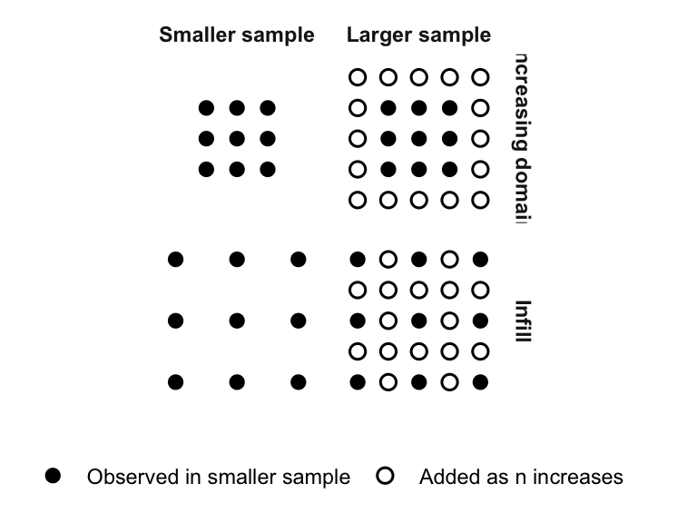
The increasing-domain framework naturally leads to the concept of a triangular array. The reason is simple: when the sample size changes, the objects that define the model also change with \(n\). In spatial models, this is particularly important because the spatial weights matrix usually depends on \(n\), and so do the endogenous spatial lags and, more generally, the random variables whose asymptotic behavior we want to study.

Definition 3.19 (Triangular Array of Random Variables) A triangular array is a collection of random variables of the form \[\left\{ X_{ni}: 1\leq i\leq n, \ n\geq 1 \right\}.\]

Equivalently, it can be displayed row by row as \[\begin{array}{cccccc} X_{11} \\ X_{21} & X_{22} \\ X_{31} & X_{32} & X_{33} \\ \vdots & \vdots & \vdots & \ddots \\ X_{n1} & X_{n2} & X_{n3} & \cdots & X_{nn}. \end{array}\]

The \(n\)th row contains \(n\) random variables: \[X_{n1},\ldots,X_{nn}.\]

The key feature is that the distributional structure may change with \(n\). In particular, the variables in row \(n\) need not have the same joint distribution as the variables in row \(m\) when \(m\neq n\).

A triangular array differs from an ordinary sequence of random variables. In a sequence, there is only one random variable associated with each index \(n\), namely \(X_n\). In a triangular array, each sample size \(n\) generates an entire row of variables, \(X_{n1},\ldots,X_{nn},\) and asymptotic results are obtained from the behavior of suitable functions of these rows. Figure 3.9 provides a visual representation.

Figure 3.9: Triangular array displayed row by row

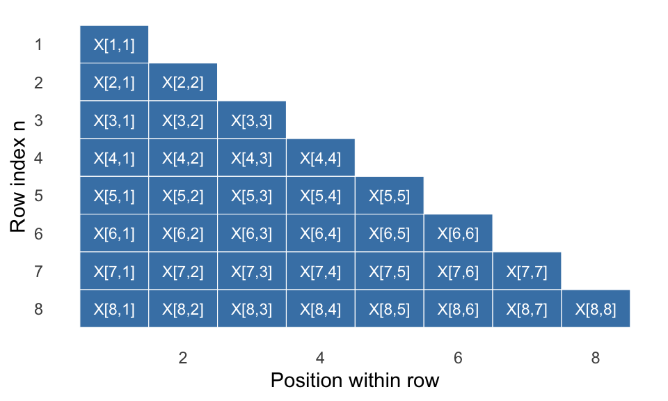
The object of interest is often a row sum or a row average. For example, the row average associated with the \(n\)th row is \[\overline X_n = \frac{1}{n}\sum_{i=1}^{n}X_{ni}.\]

When \(n=3\), this becomes \[\overline X_3 = \frac{1}{3}(X_{31}+X_{32}+X_{33}).\]

Classical limit theorems for i.i.d. sequences study averages of the form \(\frac{1}{n}\sum_{i=1}^{n}X_i.\) Triangular arrays are more general because the variables in the \(n\)th row may have distributions, variances, or dependence structures that differ from those in other rows. For that reason, the appropriate Law of Large Numbers or Central Limit Theorem must be formulated directly for triangular arrays. One should not simply apply i.i.d. results without checking whether the row structure satisfies the necessary conditions.

To motivate the basic logic, suppose we have a centered triangular array \[\{X_{ni}:1\leq i\leq n,\ n\geq1\}\] with independent observations within each row and such that \(\mathbb E(X_{ni})=0\). A triangular-array CLT typically studies the standardized row sum \[\sum_{i=1}^{n}X_{ni},\] or an equivalent normalization, under conditions such as:

• independence within each row;
• centering;
• stabilization of the row variances; and
• the requirement that no single observation dominates the row sum.

The exact theorem depends on the assumptions imposed. The important point here is not to memorize a single generic statement, but rather to understand why the usual i.i.d. CLT is often insufficient once the array structure varies with \(n\).

3.7.1 Why Triangular Arrays Arise in Spatial Econometrics

As previously mentioned, triangular arrays are important in spatial econometrics because, under increasing-domain asymptotics, the sample size \(n\) affects the structure of the spatial model itself. In particular, the spatial weights matrix generally changes with \(n\), so the data cannot usually be viewed as the first \(n\) entries of one fixed infinite sequence.

To illustrate, consider the spatial lag model written for sample size \(n\) as \[ \mathbf y_n = \rho_0\mathbf W_n\mathbf y_n + \mathbf X_n\boldsymbol\beta_0 + \boldsymbol\varepsilon_n. \]

Equivalently, \[ \mathbf y_n = \mathbf A_n(\rho_0)^{-1} \left( \mathbf X_n\boldsymbol\beta_0 + \boldsymbol\varepsilon_n \right), \]
where \(\mathbf A_n(\rho)= \mathbf I_n-\rho\mathbf W_n.\) Because \(\mathbf W_n\) depends on \(n\), the multiplier \(\mathbf A_n(\rho_0)^{-1}\) also depends on \(n\). Consequently, the random vector \(\mathbf y_n\) depends on \(n\) even when the structural parameters remain fixed. The same is true for any transformed disturbances or spatial lags built from this system.

Therefore, the observations in the \(n\)th sample should be indexed as \[ \mathbf y_n = (y_{n1},\ldots,y_{nn})^\top. \]

The notation emphasizes that the first observed unit in the sample of size \(n=10\) need not coincide with the first observed unit in the sample of size \(n=15\). More importantly, its value may differ because the entire interaction structure embodied in \(\mathbf W_n\) has changed.

Figure 3.10 illustrates this logic using a simple regular lattice. The figure does not mean that the first few labels in the larger sample must be numerically different from those in the smaller sample. Rather, it shows that once the geographical domain expands, the sample is redefined as a new row of a triangular array. In spatial models, the corresponding matrix \(\mathbf W_n\) changes with the sample, so the joint distribution of the row can change as well.

Figure 3.10: Why increasing-domain asymptotics lead naturally to triangular arrays

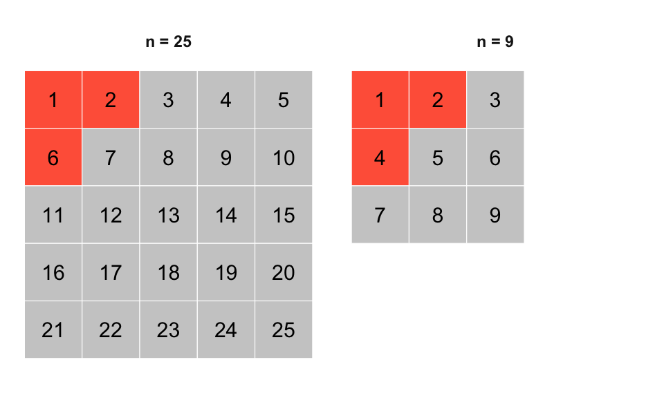
This point is important enough to state explicitly.

NoteTriangular arrays are not just a notation trick

A triangular array is not introduced merely to relabel the observations. It is introduced because, in many spatial asymptotic arguments, the row associated with sample size \(n\) is genuinely a different random object from the row associated with sample size \(m\neq n\). The dependence structure, the spatial multiplier, and sometimes even the regressor process vary with \(n\).

The triangular-array structure therefore applies not only to \(\mathbf y_n\), but often also to \(\mathbf X_n\), to transformed disturbances, and to linear or quadratic forms built from the data. That is precisely why the limit theory developed later in the chapter is formulated in terms of arrays rather than fixed i.i.d. sequences.

Finally, note that dependence within a row need not disappear merely because observations are indexed separately. In fact, in a spatial lag model the components of \(\mathbf y_n\) are generally dependent within the same row, because each observation depends, directly or indirectly, on the others through the spatial multiplier. The triangular-array notation accommodates this feature; it does not impose independence.

3.8 Bounded Matrices and Useful Lemmas for Spatial Econometrics

The transition from ordinary asymptotic theory to spatial asymptotic theory requires additional control over sequences of matrices whose dimensions grow with the sample size. In a spatial model, objects such as \(\mathbf W_n\), \((\mathbf I_n-\rho\mathbf W_n)^{-1}\), and products involving these matrices are all \(n\times n\). Their dimensions therefore increase as \(n\to\infty\).

It is not enough to know that every matrix in the sequence is finite for a particular value of \(n\). We need bounds that remain valid uniformly over all sample sizes. Otherwise, the cumulative influence represented by a row or a column of a spatial matrix could grow with \(n\) and invalidate the moment and variance bounds used in Laws of Large Numbers and Central Limit Theorems.

This section introduces the matrix restrictions used repeatedly in spatial asymptotic arguments. The central idea is straightforward: although the number of spatial units increases, the total absolute influence associated with any single row or column should remain controlled.

3.8.1 Absolute Row and Column Sums

Let \[\mathbf A_n = [a_{n,ij}]_{i,j=1}^{n}\] be a sequence of \(n\times n\) matrices. Two matrix norms are especially useful (see Definition 2.8 and Chapter 5.6 in Horn and Johnson (2012)): \[\|\mathbf A_n\|_{\infty} = \max_{1\leq i\leq n} \sum_{j=1}^{n}|a_{n,ij}| \tag{3.11}\] and \[\|\mathbf A_n\|_{1} = \max_{1\leq j\leq n} \sum_{i=1}^{n}|a_{n,ij}|. \tag{3.12}\]

The row and column norms summarize two different aspects of a matrix. For each row \(i\), define its absolute row sum as \(r_i=\sum_{j=1}^{n}|a_{ij}|\). The infinity norm is the largest of these row sums: \(\|\mathbf A\|_{\infty}=\max_{1\leq i\leq n}r_i\). Similarly, for each column \(j\), define its absolute column sum as \(c_j=\sum_{i=1}^{n}|a_{ij}|\). The one norm is the largest of these column sums: \(\|\mathbf A\|_1=\max_{1\leq j\leq n}c_j\).

The absolute values are essential. Without them, positive and negative entries could cancel. A row or column could then have a small ordinary sum even though its individual elements are large. Consider the matrix \[\mathbf A = \begin{pmatrix} 0 & 0.50 & 0.50 & 0 \\ 0.25 & 0 & -0.25 & 0.75 \\ 0 & 0.20 & 0 & 0.30 \\ -0.20 & 0 & 0.30 & 0.10 \end{pmatrix}.\]

For example, the absolute sum of the second row is \[|0.25|+|0|+|-0.25|+|0.75| = 1.25,\] whereas the absolute sum of the fourth column is \[|0|+|0.75|+|0.30|+|0.10| = 1.15.\]

Figure 3.11 compares all row and column sums. The infinity norm is the height of the largest bar in the left panel, whereas the one norm is the height of the largest bar in the right panel.

Figure 3.11: Absolute row and column sums and the corresponding matrix norms

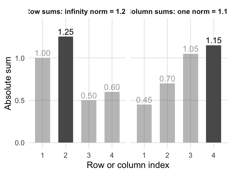
The distinction has a direct interpretation in spatial econometrics. In the spatial lag \((\mathbf W_n\mathbf y_n)_i=\sum_{j=1}^{n}w_{n,ij}y_{n,j}\), row \(i\) contains the weights used to construct the spatially weighted outcome for unit \(i\). Therefore, \(\sum_{j=1}^{n}|w_{n,ij}|\) measures the total absolute weight entering the spatial lag equation for that unit. A uniform bound on the row sums prevents any single equation from combining an increasingly large total amount of spatial influence as the sample expands.

Column \(j\), by contrast, records how the outcome of unit \(j\) enters the spatial lags of all other units. Therefore, \(\sum_{i=1}^{n}|w_{n,ij}|\) measures the total absolute influence assigned to unit \(j\) across the entire system. A uniform bound on the column sums prevents one spatial unit from becoming an increasingly influential hub as \(n\) grows.

Thus, the two conditions control spatial interaction in different directions: bounded row sums limit the total influence received by each equation, whereas bounded column sums limit the total influence transmitted by each spatial unit.

For a nonnegative row-standardized spatial weights matrix, \(\sum_{j=1}^{n}w_{n,ij}=1\), so the row sums are automatically bounded. Row standardization alone, however, does not guarantee that the column sums remain uniformly bounded. That property must be verified separately.

Definition 3.20 (Uniformly Bounded Row and Column Sums) Let \(\{\mathbf A_n\}\) be a sequence of \(n\times n\) matrices.

1. The sequence is uniformly bounded in absolute row sums if there exists a finite constant \(c_{\infty}\), independent of \(n\), such that \[\|\mathbf A_n\|_{\infty} \leq c_{\infty}\] for every \(n\).

2. The sequence is uniformly bounded in absolute column sums if there exists a finite constant \(c_1\), independent of \(n\), such that \[\|\mathbf A_n\|_1 \leq c_1\] for every \(n\).

3. The sequence is uniformly bounded in both row and column sums if both conditions hold.

The word uniformly is crucial. For every fixed \(n\), the norms of a finite matrix are finite. The asymptotic restriction requires one constant that works for the entire sequence, regardless of how large \(n\) becomes.

For a nonnegative row-standardized spatial weights matrix, \(\sum_{j=1}^{n}w_{n,ij}=1\) for every non-isolated unit, and hence \(\|\mathbf W_n\|_{\infty}\leq1\). Thus, row-sum boundedness is built into row standardization. Column-sum boundedness is a separate property and should not be inferred automatically from row standardization. It holds in many common designs, but it must follow from the structure of the spatial network or be imposed as an assumption. For example, a uniform bound on the number of units that assign positive weight to any given unit is a sufficient condition when the weights themselves are bounded.

3.8.2 Immediate Consequence for Individual Entries

Uniform boundedness of absolute row sums or column sums automatically controls every individual matrix element.

Lemma 3.5 (Uniform Bound on Matrix Entries) Suppose that \(\{\mathbf A_n\}\) is uniformly bounded either in absolute row sums or in absolute column sums. Then there exists a finite constant \(c_A\), independent of \(n\), such that \[|a_{n,ij}|\leq c_A\] for every \(i\), \(j\), and \(n\).

Proof. Suppose first that the row sums are uniformly bounded. Then, for every \(i\) and \(j\), \[|a_{n,ij}| \leq \sum_{s=1}^{n}|a_{n,is}| \leq \|\mathbf A_n\|_{\infty} \leq c_{\infty}.\]

Thus, the result holds with \(c_A=c_{\infty}\). If instead the column sums are uniformly bounded, then \[|a_{n,ij}| \leq \sum_{r=1}^{n}|a_{n,rj}| \leq \|\mathbf A_n\|_1 \leq c_1.\]

The result then holds with \(c_A=c_1\).

The converse is not true. Uniformly bounded entries do not guarantee uniformly bounded row or column sums. For example, a matrix whose entries are all equal to one has uniformly bounded entries, but each row and column sum equals \(n\).

3.8.3 Products of Uniformly Bounded Matrices

The row-sum and column-sum norms are submultiplicative: \[\|\mathbf A_n\mathbf B_n\|_{q} \leq \|\mathbf A_n\|_{q} \|\mathbf B_n\|_{q}, \qquad q\in\{1,\infty\}. \tag{3.13}\]

This property implies that uniform boundedness is preserved under multiplication.

Lemma 3.6 (Product of Uniformly Bounded Matrices) If \(\{\mathbf A_n\}\) and \(\{\mathbf B_n\}\) are uniformly bounded in absolute row sums, then \(\{\mathbf A_n\mathbf B_n\}\) is uniformly bounded in absolute row sums.

Likewise, if both sequences are uniformly bounded in absolute column sums, then their product is uniformly bounded in absolute column sums.

Proof. This proof is based on Kelejian and Prucha (1999)’s footnote 20. Let \(\mathbf D_n=\mathbf A_n\mathbf B_n\), and write its \((i,j)\)th element as \(d_{n,ij}=\sum_{r=1}^{n}a_{n,ir}b_{n,rj}\). Suppose first that \(\|\mathbf A_n\|_{\infty}\leq c_A\) and \(\|\mathbf B_n\|_{\infty}\leq c_B\) for every \(n\). For a fixed row \(i\), the triangle inequality gives \[ \begin{aligned} \sum_{j=1}^{n}|d_{n,ij}| &= \sum_{j=1}^{n} \left| \sum_{r=1}^{n}a_{n,ir}b_{n,rj} \right| \\ &\leq \sum_{j=1}^{n} \sum_{r=1}^{n} |a_{n,ir}|\,|b_{n,rj}| \\ &= \sum_{r=1}^{n} |a_{n,ir}| \sum_{j=1}^{n}|b_{n,rj}| \\ &\leq c_B \sum_{r=1}^{n}|a_{n,ir}| \\ &\leq c_Ac_B. \end{aligned} \]

The bound does not depend on \(i\) or \(n\). Taking the maximum over rows yields \[\|\mathbf A_n\mathbf B_n\|_{\infty} \leq c_Ac_B.\]

Now suppose that \(\|\mathbf A_n\|_1\leq c_A\) and \(\|\mathbf B_n\|_1\leq c_B.\) For a fixed column \(j\), \[\begin{aligned} \sum_{i=1}^{n}|d_{n,ij}| &\leq \sum_{i=1}^{n} \sum_{r=1}^{n} |a_{n,ir}|\,|b_{n,rj}| \\ &= \sum_{r=1}^{n} |b_{n,rj}| \sum_{i=1}^{n}|a_{n,ir}| \\ &\leq c_A \sum_{r=1}^{n}|b_{n,rj}| \\ &\leq c_Ac_B. \end{aligned}\] Taking the maximum over columns gives \[\|\mathbf A_n\mathbf B_n\|_1 \leq c_Ac_B.\]

Thus, uniform boundedness is preserved under matrix multiplication in either norm.

An immediate consequence is that, for any fixed positive integer \(m\), \[\|\mathbf A_n^m\|_q \leq \|\mathbf A_n\|_q^m, \qquad q\in\{1,\infty\}.\]

The qualification that \(m\) is fixed is important. The result does not provide a uniform bound when the exponent itself increases with \(n\).

3.8.4 Uniform Boundedness of the Spatial Multiplier

Spatial asymptotic arguments frequently require not only \(\mathbf W_n\), but also the spatial multiplier \(\mathbf B_n(\rho) = (\mathbf I_n-\rho\mathbf W_n)^{-1}\) to be uniformly bounded. Nonsingularity for every \(n\) does not, by itself, guarantee a uniform row- or column-sum bound as \(n\) increases. A convenient sufficient condition follows from the Neumann expansion.

Lemma 3.7 (A Sufficient Bound for the Spatial Multiplier) Let \(q\in\{1,\infty\}\). Suppose that \[\sup_n\|\mathbf W_n\|_q\leq c_W<\infty,\] and let the parameter space \(\mathcal P\) satisfy \[\sup_{\rho\in\mathcal P}|\rho| = \overline\rho\] with \[\overline\rho c_W<1.\]

Then \(\mathbf I_n-\rho\mathbf W_n\) is nonsingular and \[\sup_n\sup_{\rho\in\mathcal P} \left\| (\mathbf I_n-\rho\mathbf W_n)^{-1} \right\|_q \leq \frac{1}{1-\overline\rho c_W}.\]

Proof. For every \(n\) and every \(\rho\in\mathcal P\), \[\|\rho\mathbf W_n\|_q = |\rho|\,\|\mathbf W_n\|_q \leq \overline\rho c_W <1.\]

Therefore, the Neumann series converges: \[(\mathbf I_n-\rho\mathbf W_n)^{-1} = \sum_{s=0}^{\infty} \rho^s\mathbf W_n^s.\]

Using the triangle inequality and submultiplicativity, \[\begin{aligned} \left\| (\mathbf I_n-\rho\mathbf W_n)^{-1} \right\|_q &\leq \sum_{s=0}^{\infty} |\rho|^s\|\mathbf W_n^s\|_q \\ &\leq \sum_{s=0}^{\infty} |\rho|^s\|\mathbf W_n\|_q^s \\ &\leq \sum_{s=0}^{\infty} (\overline\rho c_W)^s \\ &= \frac{1}{1-\overline\rho c_W}. \end{aligned}\]

The final bound is finite and does not depend on \(n\) or on the particular value of \(\rho\in\mathcal P\).

For a nonnegative row-standardized matrix, \(\|\mathbf W_n\|_{\infty}\leq1\). Hence a parameter space satisfying \(|\rho|\leq\overline\rho<1\) immediately gives a uniform row-sum bound for the spatial multiplier. Obtaining a uniform column-sum bound requires the corresponding control of \(\|\mathbf W_n\|_1\) or a separate assumption.

NoteNonsingularity and uniform boundedness are different requirements

The spectral-radius condition ensures that \(\mathbf I_n-\rho\mathbf W_n\) is nonsingular for each \(n\) (see Lemma 2.1). Uniform boundedness of its inverse is stronger: it requires the inverse not to approach a singularity as \(n\) increases. Spatial asymptotic proofs often impose both properties explicitly.

3.8.5 Growth of Matrix Cross-Products

The next result is used when data or instrument matrices appear on both sides of a spatial matrix. It shows why normalizing such expressions by \(n\) is natural (see Lee 2004).

Lemma 3.8 (Growth Bound for Matrix Cross-Products) Let \(\mathbf Z_n\) be an \(n\times k\) matrix, where \(k\) is fixed, and suppose that its entries are uniformly bounded: \[|z_{n,ig}|\leq c_Z\] for all \(i\), \(g\), and \(n\). If \(\{\mathbf A_n\}\) is uniformly bounded in either absolute row sums or absolute column sums, then every element of \[\mathbf Z_n^\top\mathbf A_n\mathbf Z_n\] is \(O(n)\). Equivalently, \[\frac{1}{n} \mathbf Z_n^\top\mathbf A_n\mathbf Z_n = O(1)\] elementwise.

Proof. Fix two columns \(g\) and \(h\) of \(\mathbf Z_n\). The \((g,h)\)th element of the cross-product is \[\left[ \mathbf Z_n^\top\mathbf A_n\mathbf Z_n \right]_{gh} = \sum_{i=1}^{n} \sum_{j=1}^{n} z_{n,ig}a_{n,ij}z_{n,jh}.\]

Taking absolute values and applying the triangle inequality, \[\begin{aligned} \left| \left[ \mathbf Z_n^\top\mathbf A_n\mathbf Z_n \right]_{gh} \right| &\leq \sum_{i=1}^{n} \sum_{j=1}^{n} |z_{n,ig}|\,|a_{n,ij}|\,|z_{n,jh}| \\ &\leq c_Z^2 \sum_{i=1}^{n} \sum_{j=1}^{n}|a_{n,ij}|, \end{aligned}\] where the last inequality comes from the fact that \(\mathbf Z_n\) has bounded elements: \(|z_{n,ig}|< c_Z\). Suppose first that the row sums are uniformly bounded by \(c_A\). Then \[\begin{aligned} \sum_{i=1}^{n} \sum_{j=1}^{n}|a_{n,ij}| &= \sum_{i=1}^{n} \left( \sum_{j=1}^{n}|a_{n,ij}| \right) \\ &\leq \sum_{i=1}^{n}c_A \\ &= nc_A. \end{aligned}\]

Consequently, \[\left| \left[ \mathbf Z_n^\top\mathbf A_n\mathbf Z_n \right]_{gh} \right| \leq c_Z^2c_An.\]

If instead the column sums are uniformly bounded, the same conclusion follows by summing over columns first: \[\sum_{j=1}^{n} \left( \sum_{i=1}^{n}|a_{n,ij}| \right) \leq nc_A.\]

Thus every element is bounded by a constant times \(n\). Dividing by \(n\) yields an elementwise \(O(1)\) matrix.

This lemma establishes a growth rate only. It does not imply that \(n^{-1}\mathbf Z_n^\top\mathbf A_n\mathbf Z_n\) converges, nor that its limit is nonsingular. Those conclusions require additional assumptions.

3.8.6 Trace Bounds

Traces of spatial matrices appear in expected Hessians, variances of quadratic forms, and log-likelihood derivatives. Uniform row- or column-sum bounds imply that traces of fixed powers and quadratic trace expressions grow at most linearly with \(n\).

Lemma 3.9 (Trace Bounds) Let \(\{\mathbf A_n\}\) be uniformly bounded in either absolute row sums or absolute column sums. Then, for every fixed positive integer \(m\), \[\operatorname{tr}(\mathbf A_n^m) = O(n),\] and \[\operatorname{tr} \left( \mathbf A_n\mathbf A_n^\top \right) = O(n).\]

Proof. Suppose first that the row sums are uniformly bounded: \(\|\mathbf A_n\|_{\infty}\leq c_A\). By repeated application of Lemma 3.6, \(\|\mathbf A_n^m\|_{\infty}\leq c_A^m\) for every fixed \(m\). Hence, for every \(i\), \[|[\mathbf A_n^m]_{ii}| \leq \sum_{j=1}^{n}|[\mathbf A_n^m]_{ij}| \leq c_A^m.\]

Therefore, \[\begin{aligned} \left| \operatorname{tr}(\mathbf A_n^m) \right| &= \left| \sum_{i=1}^{n}[\mathbf A_n^m]_{ii} \right| \\ &\leq \sum_{i=1}^{n}|[\mathbf A_n^m]_{ii}| \\ &\leq nc_A^m. \end{aligned}\]

Thus, \(\operatorname{tr}(\mathbf A_n^m)=O(n)\). For the second result, observe that \[\operatorname{tr} \left( \mathbf A_n\mathbf A_n^\top \right) = \sum_{i=1}^{n} \sum_{j=1}^{n}a_{n,ij}^2.\]

For each row \(i\), \[\sum_{j=1}^{n}a_{n,ij}^2 \leq \left( \sum_{j=1}^{n}|a_{n,ij}| \right)^2 \leq c_A^2.\]

Summing over rows gives \[\operatorname{tr} \left( \mathbf A_n\mathbf A_n^\top \right) \leq nc_A^2,\] which proves the \(O(n)\) bound.

Now suppose instead that the column sums of \(\mathbf A_n\) are uniformly bounded. Then the row sums of \(\mathbf A_n^\top\) are uniformly bounded. The preceding arguments applied to \(\mathbf A_n^\top\) yield \[\operatorname{tr} \left[ (\mathbf A_n^\top)^m \right] = O(n).\]

Since \((\mathbf A_n^\top)^m=(\mathbf A_n^m)^\top\) and trace is invariant under transposition, \[\operatorname{tr}(\mathbf A_n^m) = O(n).\]

Likewise, \[\operatorname{tr} \left( \mathbf A_n^\top\mathbf A_n \right) = O(n).\]

Finally, \[\operatorname{tr} \left( \mathbf A_n^\top\mathbf A_n \right) = \operatorname{tr} \left( \mathbf A_n\mathbf A_n^\top \right),\] because both expressions equal \(\sum_{i=1}^{n}\sum_{j=1}^{n}a_{n,ij}^2\).

3.8.7 Summary of the Main Growth Bounds

Under the conditions established in this section, the following orders are available for fixed \(m\) and fixed \(k\):

Object	Order
Individual entry \(a_{n,ij}\)	\(O(1)\)
\(\|\mathbf A_n^m\|_1\) or \(\|\mathbf A_n^m\|_{\infty}\)	\(O(1)\)
\(\operatorname{tr}(\mathbf A_n^m)\)	\(O(n)\)
\(\operatorname{tr}(\mathbf A_n\mathbf A_n^\top)\)	\(O(n)\)
\(\mathbf Z_n^\top\mathbf A_n\mathbf Z_n\)	\(O(n)\) elementwise
\(n^{-1}\mathbf Z_n^\top\mathbf A_n\mathbf Z_n\)	\(O(1)\) elementwise

These results explain why normalization by \(n\) appears repeatedly in spatial moment conditions, Hessians, and variance calculations. The dimension of the matrix grows with the sample, but uniform row- and column-sum bounds prevent its aggregate contribution from growing faster than linearly in \(n\).

3.9 Linear and Quadratic Forms

Linear and quadratic forms of the disturbances appear repeatedly in the asymptotic analysis of spatial econometric estimators. For example, first-order conditions frequently contain linear forms such as \(\mathbf q_n^\top\boldsymbol\varepsilon_n\), whereas likelihood functions, variance estimators, and GMM moments often contain quadratic forms such as \(\boldsymbol\varepsilon_n^\top\mathbf A_n\boldsymbol\varepsilon_n\). Understanding their means, variances, and covariances is therefore necessary before deriving Laws of Large Numbers and Central Limit Theorems for spatial models.

3.9.1 Moments

Definition 3.21 (Linear Form) Let \(\mathbf q_n\) be a nonrandom \(n\times1\) vector and let \(\boldsymbol\varepsilon_n\) be an \(n\times1\) random vector. The scalar \[L_n = \mathbf q_n^\top\boldsymbol\varepsilon_n = \sum_{i=1}^{n}q_{ni}\varepsilon_{ni}\] is called a linear form in \(\boldsymbol\varepsilon_n\).

A linear form combines the disturbances one at a time. If \(\boldsymbol\varepsilon_n\) has mean \(\boldsymbol\mu_n\) and covariance matrix \(\boldsymbol\Sigma_n\), then \(\mathbb E(L_n)=\mathbf q_n^\top\boldsymbol\mu_n\) and \(\operatorname{Var}(L_n)=\mathbf q_n^\top\boldsymbol\Sigma_n\mathbf q_n\). When the disturbances are independent and homoskedastic with variance \(\sigma^2\), this reduces to \[\operatorname{Var}(L_n) = \sigma^2\mathbf q_n^\top\mathbf q_n = \sigma^2\sum_{i=1}^{n}q_{ni}^2.\]

A quadratic form instead combines disturbances in pairs.

Definition 3.22 (Quadratic Form) Let \(\mathbf A_n=[a_{n,ij}]\) be an \(n\times n\) matrix and let \(\boldsymbol\varepsilon_n\) be an \(n\times1\) vector. The scalar \[\begin{aligned} Q_n(\mathbf A_n) = \boldsymbol\varepsilon_n^\top \mathbf A_n \boldsymbol\varepsilon_n = \sum_{i=1}^{n}\sum_{j=1}^{n} a_{n,ij}\varepsilon_{ni}\varepsilon_{nj} \end{aligned} \tag{3.14}\]

is called a quadratic form in \(\boldsymbol\varepsilon_n\).

The matrix \(\mathbf A_n\) determines how each product \(\varepsilon_{ni}\varepsilon_{nj}\) contributes to the quadratic form. The diagonal terms involve squared disturbances, \(\sum_{i=1}^{n}a_{n,ii}\varepsilon_{ni}^2\), whereas the off-diagonal terms involve products between disturbances from different observations, \(\sum_{i=1}^{n}\sum_{j\neq i}a_{n,ij}\varepsilon_{ni}\varepsilon_{nj}\).

The definition does not require \(\mathbf A_n\) to be symmetric. Nevertheless, every quadratic form depends only on the symmetric part of its matrix. Define \[\mathbf A_n^s = \frac{1}{2} \left( \mathbf A_n+\mathbf A_n^\top \right). \tag{3.15}\]

Then \[\boldsymbol\varepsilon_n^\top \mathbf A_n \boldsymbol\varepsilon_n = \boldsymbol\varepsilon_n^\top \mathbf A_n^s \boldsymbol\varepsilon_n. \tag{3.16}\]

To verify this result, write the skew-symmetric part as \[\mathbf A_n^a = \frac{1}{2} \left( \mathbf A_n-\mathbf A_n^\top \right).\]

Since \((\mathbf A_n^a)^\top=-\mathbf A_n^a\), the scalar \(\boldsymbol\varepsilon_n^\top\mathbf A_n^a\boldsymbol\varepsilon_n\) satisfies \[\begin{aligned} \boldsymbol\varepsilon_n^\top \mathbf A_n^a \boldsymbol\varepsilon_n &= \left( \boldsymbol\varepsilon_n^\top \mathbf A_n^a \boldsymbol\varepsilon_n \right)^\top \\ &= \boldsymbol\varepsilon_n^\top (\mathbf A_n^a)^\top \boldsymbol\varepsilon_n \\ &= - \boldsymbol\varepsilon_n^\top \mathbf A_n^a \boldsymbol\varepsilon_n. \end{aligned}\]

The scalar must therefore equal zero, proving Equation 3.16.

This observation is useful in spatial econometrics because spatial weights matrices are often asymmetric after row standardization. Even in that case, the corresponding quadratic form is determined by the symmetric part of the matrix. The moment formulas developed next are standard tools in spatial asymptotic analysis (see Lee 2004).

Lemma 3.10 (First and Second Moments of a Quadratic Form) Let \(\mathbf A_n=[a_{n,ij}]\) be an \(n\times n\) nonrandom matrix and let \(\boldsymbol\varepsilon_n\) be an \(n\times1\) random vector with \(\mathbb E(\boldsymbol\varepsilon_n)=\boldsymbol\mu_n\) and \(\operatorname{Var}(\boldsymbol\varepsilon_n)=\boldsymbol\Sigma_n.\) Then \[\mathbb E\!\left[ \boldsymbol\varepsilon_n^\top \mathbf A_n \boldsymbol\varepsilon_n \right] = \operatorname{tr} \left( \mathbf A_n\boldsymbol\Sigma_n \right) + \boldsymbol\mu_n^\top \mathbf A_n \boldsymbol\mu_n. \tag{3.17}\]

Now suppose that the elements of \(\boldsymbol\varepsilon_n\) are i.i.d. and satisfy \[\mathbb E(\varepsilon_{ni})=0, \qquad \mathbb E(\varepsilon_{ni}^2)=\sigma^2, \qquad \mathbb E(\varepsilon_{ni}^4)=\mu_4<\infty.\]

Then:

1. The mean is \[\mathbb E[Q_n(\mathbf A_n)] = \sigma^2\operatorname{tr}(\mathbf A_n). \tag{3.18}\]

2. The second moment is \[\begin{aligned} \mathbb E[Q_n(\mathbf A_n)^2] = (\mu_4-3\sigma^4) \sum_{i=1}^{n}a_{n,ii}^2 + \sigma^4 \left[ \operatorname{tr}(\mathbf A_n)^2 + \operatorname{tr}(\mathbf A_n\mathbf A_n^\top) + \operatorname{tr}(\mathbf A_n^2) \right]. \end{aligned} \tag{3.19}\]

3. The variance is \[\begin{aligned} \operatorname{Var}[Q_n(\mathbf A_n)] = (\mu_4-3\sigma^4) \sum_{i=1}^{n}a_{n,ii}^2 + \sigma^4 \left[ \operatorname{tr}(\mathbf A_n\mathbf A_n^\top) + \operatorname{tr}(\mathbf A_n^2) \right]. \end{aligned} \tag{3.20}\]

Equivalently, \[\operatorname{Var}[Q_n(\mathbf A_n)] = (\mu_4-3\sigma^4) \sum_{i=1}^{n}a_{n,ii}^2 + 2\sigma^4 \operatorname{tr} \left( \mathbf A_n\mathbf A_n^s \right). \tag{3.21}\]

Proof. Let \[Q_n = Q_n(\mathbf A_n) = \boldsymbol\varepsilon_n^\top \mathbf A_n \boldsymbol\varepsilon_n.\]

Step 1: General mean formula.

By Equation 3.14, \[Q_n = \sum_{i=1}^{n}\sum_{j=1}^{n} a_{n,ij}\varepsilon_{ni}\varepsilon_{nj}.\]

Taking expectations gives \[\mathbb E(Q_n) = \sum_{i=1}^{n}\sum_{j=1}^{n} a_{n,ij} \mathbb E(\varepsilon_{ni}\varepsilon_{nj}).\]

Let \(\sigma_{n,ij}\) denote the \((i,j)\)th element of \(\boldsymbol\Sigma_n\), and let \(\mu_{n,i}\) denote the \(i\)th element of \(\boldsymbol\mu_n\). Since \[\mathbb E(\varepsilon_{ni}\varepsilon_{nj}) = \sigma_{n,ij} + \mu_{n,i}\mu_{n,j},\] we obtain \[\begin{aligned} \mathbb E(Q_n) &= \sum_{i=1}^{n}\sum_{j=1}^{n} a_{n,ij}\sigma_{n,ij} + \sum_{i=1}^{n}\sum_{j=1}^{n} a_{n,ij}\mu_{n,i}\mu_{n,j} \\ &= \operatorname{tr} \left( \mathbf A_n\boldsymbol\Sigma_n \right) + \boldsymbol\mu_n^\top \mathbf A_n \boldsymbol\mu_n. \end{aligned}\]

The trace identity follows because \(\boldsymbol\Sigma_n\) is symmetric: \[\operatorname{tr} \left( \mathbf A_n\boldsymbol\Sigma_n \right) = \sum_{i=1}^{n}\sum_{j=1}^{n} a_{n,ij}\sigma_{n,ji} = \sum_{i=1}^{n}\sum_{j=1}^{n} a_{n,ij}\sigma_{n,ij}.\]

This proves Equation 3.17.

Step 2: Mean under i.i.d. disturbances.

Under the i.i.d. assumptions, \[\mathbb E(\varepsilon_{ni}\varepsilon_{nj}) = \begin{cases} \sigma^2, & i=j,\\ 0, & i\neq j. \end{cases}\]

Therefore, \[\begin{aligned} \mathbb E(Q_n) &= \sum_{i=1}^{n}\sum_{j=1}^{n} a_{n,ij} \mathbb E(\varepsilon_{ni}\varepsilon_{nj}) \\ &= \sigma^2\sum_{i=1}^{n}a_{n,ii} \\ &= \sigma^2\operatorname{tr}(\mathbf A_n). \end{aligned}\]

This proves Equation 3.18.

Step 3: Second moment under i.i.d. disturbances.

Squaring the quadratic form yields \[Q_n^2 = \sum_{i=1}^{n} \sum_{j=1}^{n} \sum_{k=1}^{n} \sum_{\ell=1}^{n} a_{n,ij}a_{n,k\ell} \varepsilon_{ni}\varepsilon_{nj} \varepsilon_{nk}\varepsilon_{n\ell}.\]

Hence, \[\mathbb E(Q_n^2) = \sum_{i=1}^{n} \sum_{j=1}^{n} \sum_{k=1}^{n} \sum_{\ell=1}^{n} a_{n,ij}a_{n,k\ell} \mathbb E \left( \varepsilon_{ni}\varepsilon_{nj} \varepsilon_{nk}\varepsilon_{n\ell} \right).\]

Because the disturbances are independent and have mean zero, this expectation is nonzero only when every distinct index appears at least twice. There are four possible configurations:

1. \(i=j=k=\ell\), contributing the fourth moment \(\mathbb E(\epsilon_i\epsilon_j\epsilon_k\epsilon_l)=\mathbb E(\epsilon_i^4)=\mu_4\);
2. \(i=j\neq k=\ell\), contributing \(\mathbb E(\epsilon_i\epsilon_j\epsilon_k\epsilon_l)=\mathbb E(\epsilon_i^2)\mathbb E(\epsilon_k^2)=\sigma^4\);
3. \(i=k\neq j=\ell\), contributing \(\mathbb E(\epsilon_i\epsilon_j\epsilon_k\epsilon_l)=\mathbb E(\epsilon_i^2)\mathbb E(\epsilon_j^2)=\sigma^4\);
4. \(i=\ell\neq j=k\), contributing \(\mathbb E(\epsilon_i\epsilon_j\epsilon_k\epsilon_l)=\mathbb E(\epsilon_i^2)\mathbb E(\epsilon_j^2)=\sigma^4\).

Consequently, \[\begin{aligned} \mathbb E(Q_n^2) = \mu_4\sum_{i=1}^{n}a_{n,ii}^2 + \sigma^4 \sum_{i=1}^{n}\sum_{j\neq i} a_{n,ii}a_{n,jj} + \sigma^4 \sum_{i=1}^{n}\sum_{j\neq i} a_{n,ij}^2 + \sigma^4 \sum_{i=1}^{n}\sum_{j\neq i} a_{n,ij}a_{n,ji}. \end{aligned} \tag{3.22}\]

Each double sum can be written using traces. First, \[\sum_{i=1}^{n}\sum_{j\neq i} a_{n,ii}a_{n,jj} = \operatorname{tr}(\mathbf A_n)^2 - \sum_{i=1}^{n}a_{n,ii}^2.\]

Second, \[\sum_{i=1}^{n}\sum_{j\neq i} a_{n,ij}^2 = \operatorname{tr} \left( \mathbf A_n\mathbf A_n^\top \right) - \sum_{i=1}^{n}a_{n,ii}^2.\]

Third, \[\sum_{i=1}^{n}\sum_{j\neq i} a_{n,ij}a_{n,ji} = \operatorname{tr}(\mathbf A_n^2) - \sum_{i=1}^{n}a_{n,ii}^2.\]

Substituting these three identities into Equation 3.22 gives \[\begin{aligned} \mathbb E(Q_n^2) = (\mu_4-3\sigma^4) \sum_{i=1}^{n}a_{n,ii}^2 + \sigma^4 \left[ \operatorname{tr}(\mathbf A_n)^2 + \operatorname{tr} \left( \mathbf A_n\mathbf A_n^\top \right) + \operatorname{tr}(\mathbf A_n^2) \right]. \end{aligned}\]

This proves Equation 3.19.

Step 4: Variance under i.i.d. disturbances.

By definition, \[\operatorname{Var}(Q_n) = \mathbb E(Q_n^2) - [\mathbb E(Q_n)]^2.\]

From Equation 3.18, \[[\mathbb E(Q_n)]^2 = \sigma^4\operatorname{tr}(\mathbf A_n)^2.\]

Subtracting this term from Equation 3.19 yields Equation 3.20.

Finally, from Equation 3.15, \[\begin{aligned} 2\operatorname{tr} \left( \mathbf A_n\mathbf A_n^s \right) &= \operatorname{tr} \left[ \mathbf A_n (\mathbf A_n+\mathbf A_n^\top) \right] \\ &= \operatorname{tr}(\mathbf A_n^2) + \operatorname{tr} \left( \mathbf A_n\mathbf A_n^\top \right). \end{aligned}\]

Substitution gives Equation 3.21.

The term \(\mu_4-3\sigma^4\) measures the departure of the fourth moment from its normal-distribution value. For normally distributed disturbances, \(\mu_4=3\sigma^4\), and this term vanishes. Under nonnormality, the diagonal elements of \(\mathbf A_n\) therefore play an additional role in the variance of the quadratic form.

Two special cases help interpret the result.

Sum of squared disturbances. If \(\mathbf A_n=\mathbf I_n\), then \[Q_n(\mathbf I_n) = \sum_{i=1}^{n}\varepsilon_{ni}^2.\]

The formulas above imply \[\mathbb E[Q_n(\mathbf I_n)] = n\sigma^2\] and \[\operatorname{Var}[Q_n(\mathbf I_n)] = n(\mu_4-\sigma^4).\]

Spatial cross-products. If \(\mathbf A_n=\mathbf W_n\) and \(\mathbf W_n\) has a zero diagonal, then \[\mathbb E \left( \boldsymbol\varepsilon_n^\top \mathbf W_n \boldsymbol\varepsilon_n \right) = 0.\]

Its variance is \[\sigma^4 \left[ \operatorname{tr} \left( \mathbf W_n\mathbf W_n^\top \right) + \operatorname{tr}(\mathbf W_n^2) \right].\]

Thus, even when the mean is zero, the quadratic form is random and its variance depends on the pattern and intensity of the spatial links represented by \(\mathbf W_n\).

Lemma 3.11 (Gaussian Quadratic Forms) Suppose \[\boldsymbol\varepsilon_n \sim \mathcal N \left( \boldsymbol\mu_n, \boldsymbol\Sigma_n \right).\]

Let \(\mathbf A_n\) and \(\mathbf B_n\) be nonrandom \(n\times n\) matrices, and let \(\mathbf A_n^s\) and \(\mathbf B_n^s\) denote their symmetric parts. Then \[ \begin{aligned} \operatorname{Cov} \left( \boldsymbol\varepsilon_n^\top \mathbf A_n \boldsymbol\varepsilon_n, \boldsymbol\varepsilon_n^\top \mathbf B_n \boldsymbol\varepsilon_n \right) = 2\operatorname{tr} \left( \mathbf A_n^s \boldsymbol\Sigma_n \mathbf B_n^s \boldsymbol\Sigma_n \right) + 4\boldsymbol\mu_n^\top \mathbf A_n^s \boldsymbol\Sigma_n \mathbf B_n^s \boldsymbol\mu_n. \end{aligned} \tag{3.23}\]

Setting \(\mathbf B_n=\mathbf A_n\) gives \[ \begin{aligned} \operatorname{Var} \left( \boldsymbol\varepsilon_n^\top \mathbf A_n \boldsymbol\varepsilon_n \right) = 2\operatorname{tr} \left( \mathbf A_n^s \boldsymbol\Sigma_n \mathbf A_n^s \boldsymbol\Sigma_n \right) + 4\boldsymbol\mu_n^\top \mathbf A_n^s \boldsymbol\Sigma_n \mathbf A_n^s \boldsymbol\mu_n. \end{aligned} \tag{3.24}\]

The formulas in Lemma 3.11 are standard Gaussian quadratic-form identities. The symmetric parts appear because of Equation 3.16. In the centered homoskedastic case, \[\boldsymbol\mu_n=\mathbf 0, \qquad \boldsymbol\Sigma_n=\sigma^2\mathbf I_n,\]

Equation 3.24 simplifies to \[\operatorname{Var} \left( \boldsymbol\varepsilon_n^\top \mathbf A_n \boldsymbol\varepsilon_n \right) = 2\sigma^4 \operatorname{tr} \left[ (\mathbf A_n^s)^2 \right].\]

Because \[2\operatorname{tr} \left[ (\mathbf A_n^s)^2 \right] = \operatorname{tr} \left( \mathbf A_n\mathbf A_n^\top \right) + \operatorname{tr}(\mathbf A_n^2),\] this expression agrees with Equation 3.20 when \(\mu_4=3\sigma^4\).

We next need cross-moments involving a linear form and one or two quadratic forms. These quantities appear when deriving covariances among score components or GMM moments.

Lemma 3.12 (Cross-Moments of Linear and Quadratic Forms) Let \(\mathbf q_n\) be a nonrandom \(n\times1\) vector, and let \(\mathbf A_n\) and \(\mathbf B_n\) be nonrandom \(n\times n\) matrices. Suppose the elements of \(\boldsymbol\varepsilon_n\) are i.i.d. and satisfy \[\mathbb E(\varepsilon_{ni})=0, \qquad \mathbb E(\varepsilon_{ni}^2)=\sigma^2, \qquad \mathbb E(\varepsilon_{ni}^3)=\mu_3, \qquad \mathbb E(\varepsilon_{ni}^4)=\mu_4<\infty.\]

Then:

1. The linear–quadratic cross-moment is \[\mathbb E \left[ (\mathbf q_n^\top\boldsymbol\varepsilon_n) (\boldsymbol\varepsilon_n^\top \mathbf A_n \boldsymbol\varepsilon_n) \right] = \mu_3 \mathbf q_n^\top \operatorname{diag}(\mathbf A_n), \tag{3.25}\] where \(\operatorname{diag}(\mathbf A_n)\) denotes the vector containing the diagonal elements of \(\mathbf A_n\).

2. The product moment of two quadratic forms is \[\begin{aligned} &\mathbb E \left[ Q_n(\mathbf A_n)Q_n(\mathbf B_n) \right] \\ &\quad= (\mu_4-3\sigma^4) \operatorname{diag}(\mathbf A_n)^\top \operatorname{diag}(\mathbf B_n) \\ &\qquad+ \sigma^4 \left[ \operatorname{tr}(\mathbf A_n) \operatorname{tr}(\mathbf B_n) + \operatorname{tr} \left( \mathbf A_n\mathbf B_n^\top \right) + \operatorname{tr} \left( \mathbf A_n\mathbf B_n \right) \right]. \end{aligned} \tag{3.26}\]

3. Their covariance is \[\begin{aligned} &\operatorname{Cov} \left[ Q_n(\mathbf A_n), Q_n(\mathbf B_n) \right] \\ &\quad= (\mu_4-3\sigma^4) \operatorname{diag}(\mathbf A_n)^\top \operatorname{diag}(\mathbf B_n) \\ &\qquad+ \sigma^4 \left[ \operatorname{tr} \left( \mathbf A_n\mathbf B_n^\top \right) + \operatorname{tr} \left( \mathbf A_n\mathbf B_n \right) \right]. \end{aligned} \tag{3.27}\]

Equivalently, \[\begin{aligned} &\operatorname{Cov} \left[ Q_n(\mathbf A_n), Q_n(\mathbf B_n) \right] \\ &\quad= (\mu_4-3\sigma^4) \operatorname{diag}(\mathbf A_n)^\top \operatorname{diag}(\mathbf B_n) + 2\sigma^4 \operatorname{tr} \left( \mathbf A_n\mathbf B_n^s \right). \end{aligned} \tag{3.28}\]

Proof. Define \[L_n = \mathbf q_n^\top\boldsymbol\varepsilon_n = \sum_{r=1}^{n}q_{nr}\varepsilon_{nr}.\]

Step 1: Linear–quadratic cross-moment.

Using Equation 3.14, \[L_nQ_n(\mathbf A_n) = \sum_{r=1}^{n} \sum_{i=1}^{n} \sum_{j=1}^{n} q_{nr}a_{n,ij} \varepsilon_{nr}\varepsilon_{ni}\varepsilon_{nj}.\]

Taking expectations gives \[\mathbb E[L_nQ_n(\mathbf A_n)] = \sum_{r=1}^{n} \sum_{i=1}^{n} \sum_{j=1}^{n} q_{nr}a_{n,ij} \mathbb E (\varepsilon_{nr}\varepsilon_{ni}\varepsilon_{nj}).\]

Because the disturbances are independent and centered, the expectation of the triple product is zero unless \(r=i=j\). If one index differs from the other two, the corresponding disturbance appears only once and has expectation zero. Therefore, \[\mathbb E (\varepsilon_{nr}\varepsilon_{ni}\varepsilon_{nj}) = \begin{cases} \mu_3, & r=i=j,\\ 0, & \text{otherwise}. \end{cases}\]

It follows that \[\begin{aligned} \mathbb E[L_nQ_n(\mathbf A_n)] &= \mu_3\sum_{i=1}^{n}q_{ni}a_{n,ii} \\ &= \mu_3 \mathbf q_n^\top \operatorname{diag}(\mathbf A_n). \end{aligned}\]

This proves Equation 3.25.

Step 2: Product of two quadratic forms.

Expanding their product yields \[\begin{aligned} Q_n(\mathbf A_n)Q_n(\mathbf B_n) = \sum_{i=1}^{n} \sum_{j=1}^{n} \sum_{k=1}^{n} \sum_{\ell=1}^{n} a_{n,ij}b_{n,k\ell} \times \varepsilon_{ni}\varepsilon_{nj} \varepsilon_{nk}\varepsilon_{n\ell}. \end{aligned}\]

The same four index configurations used in the proof of Lemma 3.10 are the only ones with nonzero expectations. Therefore, \[\begin{aligned} \mathbb E \left[ Q_n(\mathbf A_n)Q_n(\mathbf B_n) \right] = \mu_4\sum_{i=1}^{n}a_{n,ii}b_{n,ii} + \sigma^4 \sum_{i=1}^{n}\sum_{j\neq i} a_{n,ii}b_{n,jj} + \sigma^4 \sum_{i=1}^{n}\sum_{j\neq i} a_{n,ij}b_{n,ij} + \sigma^4 \sum_{i=1}^{n}\sum_{j\neq i} a_{n,ij}b_{n,ji}. \end{aligned}\]

The four relevant identities are \[\sum_{i=1}^{n}a_{n,ii}b_{n,ii} = \operatorname{diag}(\mathbf A_n)^\top \operatorname{diag}(\mathbf B_n),\]

\[\sum_{i=1}^{n}\sum_{j\neq i} a_{n,ii}b_{n,jj} = \operatorname{tr}(\mathbf A_n) \operatorname{tr}(\mathbf B_n) - \sum_{i=1}^{n}a_{n,ii}b_{n,ii},\]

\[\sum_{i=1}^{n}\sum_{j\neq i} a_{n,ij}b_{n,ij} = \operatorname{tr} \left( \mathbf A_n\mathbf B_n^\top \right) - \sum_{i=1}^{n}a_{n,ii}b_{n,ii},\] and \[\sum_{i=1}^{n}\sum_{j\neq i} a_{n,ij}b_{n,ji} = \operatorname{tr} \left( \mathbf A_n\mathbf B_n \right) - \sum_{i=1}^{n}a_{n,ii}b_{n,ii}.\]

Substituting these identities and collecting the three subtracted diagonal terms produces Equation 3.26.

Step 3: Covariance of two quadratic forms.

From Equation 3.18, \[\mathbb E[Q_n(\mathbf A_n)] = \sigma^2\operatorname{tr}(\mathbf A_n)\] and \[\mathbb E[Q_n(\mathbf B_n)] = \sigma^2\operatorname{tr}(\mathbf B_n).\]

Thus, \[\mathbb E[Q_n(\mathbf A_n)] \mathbb E[Q_n(\mathbf B_n)] = \sigma^4 \operatorname{tr}(\mathbf A_n) \operatorname{tr}(\mathbf B_n).\]

Subtracting this product from Equation 3.26 gives Equation 3.27.

Finally, \[\mathbf B_n^s = \frac{1}{2} (\mathbf B_n+\mathbf B_n^\top)\] implies \[2\operatorname{tr} \left( \mathbf A_n\mathbf B_n^s \right) = \operatorname{tr}(\mathbf A_n\mathbf B_n) + \operatorname{tr} \left( \mathbf A_n\mathbf B_n^\top \right),\] which proves Equation 3.28.

Several implications are useful later:

• If the disturbance distribution is symmetric around zero, then \(\mu_3=0\), so a centered linear form is uncorrelated with a quadratic form.
• Under normality, \(\mu_3=0\) and \(\mu_4=3\sigma^4\), eliminating both the skewness term and the excess-fourth-moment term.
• If \(\mathbf A_n\) and \(\mathbf B_n\) have zero diagonals, the term involving \(\mu_4-3\sigma^4\) disappears even without normality.
• The traces in Equation 3.27 determine the covariance generated by the overlap between the weighting patterns in \(\mathbf A_n\) and \(\mathbf B_n\).

These moment identities provide the building blocks for the Laws of Large Numbers and Central Limit Theorems for linear and quadratic forms developed in the next sections.

3.9.2 Law of Large Numbers for Linear and Quadratic Forms

The usual Law of Large Numbers concerns averages of random variables. Spatial econometric estimators, however, frequently involve objects such as \[\frac{1}{n} \boldsymbol\varepsilon_n^\top \mathbf A_n \boldsymbol\varepsilon_n\] and \[\frac{1}{\sqrt n} \mathbf c_n^\top \mathbf A_n \boldsymbol\varepsilon_n,\] where the matrix \(\mathbf A_n\) may depend on the spatial weights matrix and therefore changes with the sample size. We consequently need results that play the role of a Law of Large Numbers for these linear and quadratic forms.

The basic argument has two parts. First, boundedness conditions on \(\mathbf A_n\) control the order of the mean and variance. Second, Chebyshev’s inequality shows that the normalized random form becomes close to its expectation. This is the central idea behind the following result, which is closely related to the quadratic-form arguments used in spatial asymptotic theory; see, for example, Kelejian and Prucha (1999).

Lemma 3.13 (Concentration and Order of a Quadratic Form) Let \(\{\mathbf A_n\}\) be a sequence of nonrandom \(n\times n\) matrices whose absolute row sums and absolute column sums are uniformly bounded. Let \[\boldsymbol\varepsilon_n = (\varepsilon_{n1},\ldots,\varepsilon_{nn})^\top,\] where, for every \(n\), the elements \(\varepsilon_{n1},\ldots,\varepsilon_{nn}\) are i.i.d. and satisfy \[\mathbb E(\varepsilon_{ni})=0, \qquad \mathbb E(\varepsilon_{ni}^2)=\sigma_0^2, \qquad \mathbb E(\varepsilon_{ni}^4)=\mu_4<\infty. \]

Define \[Q_n = \boldsymbol\varepsilon_n^\top \mathbf A_n \boldsymbol\varepsilon_n. \]

Then:

1. The expectation grows at most linearly: \(\mathbb E(Q_n)=O(n).\)

2. The variance grows at most linearly: \(\operatorname{Var}(Q_n)=O(n).\)

3. The centered quadratic form has stochastic order \(\sqrt n\): \(Q_n-\mathbb E(Q_n) =O_p(\sqrt n).\)

4. The quadratic form divided by \(n\) concentrates around its normalized expectation: \[ \frac{Q_n}{n} - \frac{\mathbb E(Q_n)}{n} = o_p(1). \tag{3.29}\]

5. The uncentered quadratic form satisfies \(Q_n=O_p(n).\)

Proof. We prove each statement in turn.

Step 1: Order of the expectation.

By Equation 3.18, \(\mathbb E(Q_n)=\sigma_0^2\operatorname{tr}(\mathbf A_n)\). The uniform row- and column-sum bounds imply, by Lemma 3.9, that \(\operatorname{tr}(\mathbf A_n)=O(n)\). Since \(\sigma_0^2\) is fixed, \[\mathbb E(Q_n) = \sigma_0^2O(n) = O(n).\]

This proves part 1.

Step 2: Order of the variance.

By Equation 3.20, \[\begin{aligned} \operatorname{Var}(Q_n) = (\mu_4-3\sigma_0^4) \sum_{i=1}^{n}a_{n,ii}^2 + \sigma_0^4 \left[ \operatorname{tr} (\mathbf A_n\mathbf A_n^\top) + \operatorname{tr}(\mathbf A_n^2) \right]. \end{aligned}\]

We bound the three matrix quantities separately.

Because the absolute row sums are uniformly bounded, there exists a finite constant \(c_A\) such that \(\sum_{j=1}^{n}|a_{n,ij}|\leq c_A\) for every \(i\) and \(n\). In particular, \(|a_{n,ii}|\leq c_A\) (by Lemma 3.5). Therefore, \[\sum_{i=1}^{n}a_{n,ii}^2 \leq nc_A^2 = O(n).\]

Moreover, Lemma 3.9 gives \[\operatorname{tr} (\mathbf A_n\mathbf A_n^\top) = O(n)\] and \[\operatorname{tr}(\mathbf A_n^2) = O(n).\]

Applying the triangle inequality to the variance expression yields \[ \begin{aligned} \operatorname{Var}(Q_n) \leq |\mu_4-3\sigma_0^4| \sum_{i=1}^{n}a_{n,ii}^2 + \sigma_0^4 \left| \operatorname{tr} (\mathbf A_n\mathbf A_n^\top) \right| + \sigma_0^4 \left| \operatorname{tr}(\mathbf A_n^2) \right| = O(n). \end{aligned}\]

This proves part 2.

Step 3: Stochastic order of the centered form. Let \[R_n = \frac{Q_n-\mathbb E(Q_n)}{\sqrt n}.\]

Then \(\mathbb E(R_n)=0\) and \(\operatorname{Var}(R_n)=\frac{1}{n}\operatorname{Var}(Q_n)\). Part 2 implies that there is a finite constant \(C\) such that, for all sufficiently large \(n\), \(\operatorname{Var}(R_n)\leq C\). For any \(M>0\), Chebyshev’s inequality (Theorem 3.28) gives \[\Pr(|R_n|>M) \leq \frac{\operatorname{Var}(R_n)}{M^2} \leq \frac{C}{M^2}.\]

Given any \(\eta>0\), choose \(M\) large enough that \(C/M^2<\eta\). By Definition 3.15 it follows that \[R_n=O_p(1).\]

Equivalently, \[Q_n-\mathbb E(Q_n) = O_p(\sqrt n).\]

This proves part 3.

Step 4: Concentration after division by \(n\).

From part 3, \[\frac{Q_n-\mathbb E(Q_n)}{n} = \frac{1}{\sqrt n} \frac{Q_n-\mathbb E(Q_n)}{\sqrt n}.\]

The second factor is \(O_p(1)\) and the first factor converges deterministically to zero. Therefore, \[\frac{Q_n-\mathbb E(Q_n)}{n} = o_p(1).\]

The same result follows directly from Chebyshev’s inequality. For every \(\delta>0\), \[\begin{aligned} \Pr\left( \left| \frac{Q_n-\mathbb E(Q_n)}{n} \right|>\delta \right) &\leq \frac{\operatorname{Var}(Q_n)}{n^2\delta^2} \\ &= O\left(\frac{1}{n}\right) \longrightarrow 0. \end{aligned}\]

This proves part 4.

Step 5: Order of the uncentered form.

Write \[\frac{Q_n}{n} = \frac{Q_n-\mathbb E(Q_n)}{n} + \frac{\mathbb E(Q_n)}{n}.\]

By part 4, the first term is \(o_p(1)\). By part 1, the second term is \(O(1)\). Hence, \[\frac{Q_n}{n} = O_p(1), \] which is equivalent to \(Q_n=O_p(n).\)

This completes the proof.

The most important conclusion is Equation 3.29. It says that sampling variation in \(Q_n/n\) disappears asymptotically. It does not, by itself, say that \(Q_n/n\) converges to a fixed constant. For that stronger conclusion, the normalized expectation must also converge.

Corollary 3.3 (Probability Limit of a Normalized Quadratic Form) Under the conditions of Lemma 3.13, suppose additionally that \[\frac{1}{n}\operatorname{tr}(\mathbf A_n) \longrightarrow \tau_A\] for some finite constant \(\tau_A\). Then \[\frac{1}{n} \boldsymbol\varepsilon_n^\top \mathbf A_n \boldsymbol\varepsilon_n \overset{p}{\longrightarrow} \sigma_0^2\tau_A. \tag{3.30}\]

Proof. By Equation 3.18, \[\frac{1}{n}\mathbb E(Q_n) = \sigma_0^2 \frac{1}{n}\operatorname{tr}(\mathbf A_n).\]

The additional assumption therefore implies \[\frac{1}{n}\mathbb E(Q_n) \longrightarrow \sigma_0^2\tau_A.\]

By Equation 3.29, \[\frac{Q_n}{n} - \frac{\mathbb E(Q_n)}{n} \overset{p}{\longrightarrow} 0.\]

Combining the deterministic convergence of the normalized expectation with this convergence in probability gives \[\frac{Q_n}{n} \overset{p}{\longrightarrow} \sigma_0^2\tau_A.\]

A useful special case occurs when every \(\mathbf A_n\) has a zero diagonal. In that case, \[\operatorname{tr}(\mathbf A_n)=0\] for every \(n\), and hence \[\frac{1}{n} \boldsymbol\varepsilon_n^\top \mathbf A_n \boldsymbol\varepsilon_n \overset{p}{\longrightarrow} 0.\]

This result is often useful when \(\mathbf A_n\) is a spatial weights matrix with zero diagonal. Notice, however, that the unnormalized quadratic form need not converge to zero. Its centered stochastic variation is generally of order \(\sqrt n\).

Figure 3.12 illustrates the concentration result for a circular spatial weights matrix. Each boxplot is based on repeated samples of \(\frac{1}{n}\boldsymbol\varepsilon_n^\top\mathbf W_n\boldsymbol\varepsilon_n\). Because \(\mathbf W_n\) has a zero diagonal, the expectation is zero. As \(n\) increases, the distribution becomes increasingly concentrated around zero.

Figure 3.12: Concentration of a normalized spatial quadratic form around its expectation

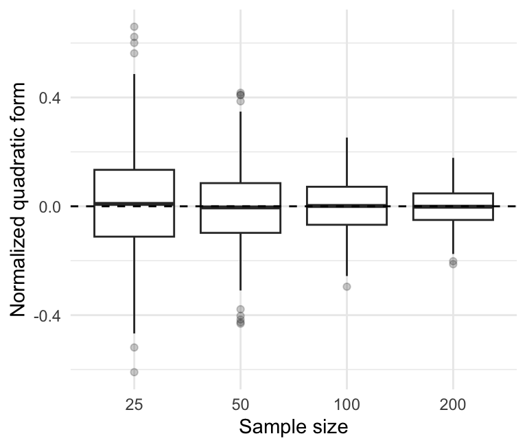
Obviously, the figure is illustrative rather than a proof. The theorem establishes the concentration result for every matrix sequence satisfying its assumptions, not only for the circular matrix used in the simulation.

3.9.3 A Related Result for Linear Forms

Linear forms also appear repeatedly in spatial estimation. For example, score vectors and sample moments often contain expressions of the form \[\frac{1}{\sqrt n} \mathbf c_n^\top \mathbf A_n \boldsymbol\varepsilon_n.\]

The following lemma shows how the size of the deterministic vector \(\mathbf c_n\) controls the stochastic order of this expression.

Lemma 3.14 (Stochastic Order of a Spatial Linear Form) Let \(\{\mathbf A_n\}\) be a sequence of nonrandom \(n\times n\) matrices such that \[\sup_n\|\mathbf A_n\|_2<\infty,\] where \(\|\cdot\|_2\) is the spectral matrix norm. Let \(\mathbf c_n\) be a nonrandom \(n\times1\) vector, and let the elements of \(\boldsymbol\varepsilon_n\) be independent with \[\mathbb E(\varepsilon_{ni})=0, \qquad \mathbb E(\varepsilon_{ni}^2)=\sigma_0^2.\]

Define \[L_n = \frac{1}{\sqrt n} \mathbf c_n^\top \mathbf A_n \boldsymbol\varepsilon_n.\]

Then:

1. If \(\frac{1}{n}\mathbf c_n^\top\mathbf c_n \longrightarrow 0,\) then \(L_n=o_p(1).\)

2. If \(\frac{1}{n}\mathbf c_n^\top\mathbf c_n =O(1),\) then \(L_n=O_p(1).\)

Proof. Since \(\mathbb E(\boldsymbol\varepsilon_n)=\mathbf0\), \(\mathbb E(L_n)=0\). Because \(\operatorname{Var}(\boldsymbol\varepsilon_n)=\sigma_0^2\mathbf I_n\), we have \[\begin{aligned} \operatorname{Var}(L_n) &= \frac{1}{n} \mathbf c_n^\top \mathbf A_n \operatorname{Var}(\boldsymbol\varepsilon_n) \mathbf A_n^\top \mathbf c_n \\ &= \frac{\sigma_0^2}{n} \mathbf c_n^\top \mathbf A_n\mathbf A_n^\top \mathbf c_n. \end{aligned}\]

For every conformable vector \(\mathbf c_n\), \[\mathbf c_n^\top \mathbf A_n\mathbf A_n^\top \mathbf c_n \leq \|\mathbf A_n\mathbf A_n^\top\|_2 \mathbf c_n^\top\mathbf c_n.\]

Moreover, \[\|\mathbf A_n\mathbf A_n^\top\|_2 = \|\mathbf A_n\|_2^2.\]

Since the spectral norms are uniformly bounded, there exists a finite constant \(c_A\) such that \(\|\mathbf A_n\|_2\leq c_A\) for every \(n\). Therefore, \[\operatorname{Var}(L_n) \leq \sigma_0^2c_A^2 \frac{\mathbf c_n^\top\mathbf c_n}{n}. \tag{3.31}\]

Suppose first that \[\frac{\mathbf c_n^\top\mathbf c_n}{n} \longrightarrow0.\]

Then Equation 3.31 implies \[\operatorname{Var}(L_n) \longrightarrow0.\]

For every \(\delta>0\), Chebyshev’s inequality gives \[\Pr(|L_n|>\delta) \leq \frac{\operatorname{Var}(L_n)}{\delta^2} \longrightarrow0.\]

Hence, \[L_n=o_p(1).\]

Now suppose that \[\frac{\mathbf c_n^\top\mathbf c_n}{n} =O(1).\]

Then Equation 3.31 implies \[\operatorname{Var}(L_n)=O(1).\]

Thus there exists a finite constant \(C\) such that, for all sufficiently large \(n\), \[\operatorname{Var}(L_n)\leq C.\]

For every \(M>0\), Chebyshev’s inequality gives \[\Pr(|L_n|>M) \leq \frac{C}{M^2}.\]

Given any \(\eta>0\), choose \(M\) large enough that \(C/M^2<\eta\). Therefore, \[L_n=O_p(1).\]

This proves both statements.

Uniform bounds on both the absolute row and column sums of \(\mathbf A_n\) imply a uniform spectral-norm bound because \[ \|\mathbf A_n\|_2 \leq \sqrt{ \|\mathbf A_n\|_1 \|\mathbf A_n\|_\infty }. \tag{3.32}\]

Thus, the conditions commonly imposed on spatial weights matrices are also sufficient for applying Lemma 3.14.

The two results in this section perform different roles. The quadratic-form lemma gives a Law of Large Numbers after division by \(n\). The linear-form lemma controls the order of a score-like expression after division by \(\sqrt n\). Together, they provide the basic stochastic rates used in the consistency and asymptotic-normality arguments developed later in the chapter.

3.10 Central Limit Theorems for Spatial Models

The role of triangular arrays in spatial econometrics was already explained in Section 3.7 and Section 3.7.1. We do not repeat that discussion here. Instead, this section develops the sequence of central limit theorems that is used in spatial estimation and testing.

The historical development is useful because each theorem solves a problem that the preceding result cannot handle.

1. The linear-form theorem used by Kelejian and Prucha (1998) and Kelejian and Prucha (1999) covers vectors such as \[ \frac{1}{\sqrt n} \mathbf A_n^{\top}\boldsymbol\varepsilon_n. \] This is the natural form of an IV moment or a score that is linear in the innovations.

2. The scalar theorem in Kelejian and Prucha (2001) adds a quadratic component: \[ \boldsymbol\varepsilon_n^{\top} \mathbf B_n \boldsymbol\varepsilon_n {}+ \mathbf b_n^{\top}\boldsymbol\varepsilon_n. \]

   This extension is needed for Moran-type statistics, quadratic GMM moments, and likelihood scores containing both linear and quadratic terms.

3. Theorem A.1 in Kelejian and Prucha (2010) extends the scalar result to a fixed-dimensional vector of linear–quadratic forms. This is the form needed for a score vector or a vector of GMM moment conditions.

The proofs also evolve. The linear theorem follows from the Lindeberg–Feller theorem and the Cramér–Wold device. The scalar linear–quadratic theorem requires a martingale-difference representation because the products inside a quadratic form are not independent. The vector result then follows from the scalar theorem and another application of Cramér–Wold.

NoteRoad map

The logical sequence is \[ \text{triangular-array Lindeberg--Feller} \Longrightarrow \text{vector linear-form CLT} \] and \[ \text{martingale CLT} \Longrightarrow \text{scalar linear--quadratic CLT} \Longrightarrow \text{vector linear--quadratic CLT}. \]

3.10.1 A Triangular-Array Version of Lindeberg–Feller

The univariate Lindeberg–Feller theorem in Theorem 3.15 was stated for a single sequence. Spatial asymptotics require its triangular-array version.

Theorem 3.20 (Lindeberg–Feller CLT for triangular arrays) For every \(n\), let \(X_{n1},\ldots,X_{nk_n}\) be independent random variables such that \[ \mathbb E(X_{ni})=0. \]

Define \[ s_n^2 = \sum_{i=1}^{k_n} \operatorname{Var}(X_{ni}), \] and suppose that \(s_n^2>0\) for all sufficiently large \(n\). If, for every \(\epsilon>0\), \[ \frac{1}{s_n^2} \sum_{i=1}^{k_n} \mathbb E \left[ X_{ni}^2 \mathbf 1 \left\{ |X_{ni}|>\epsilon s_n \right\} \right] \longrightarrow 0, \tag{3.33}\] then \[ \frac{1}{s_n} \sum_{i=1}^{k_n}X_{ni} \overset{d}{\longrightarrow} \mathcal N(0,1). \tag{3.34}\]

This is the triangular-array counterpart of Theorem 3.15. The distinction is that both the random variables and the number of terms in each row may change with \(n\).

The Lyapunov condition remains a convenient sufficient condition.

Theorem 3.21 (Lyapunov CLT for triangular arrays) For every \(n\), let \(X_{n1},\ldots,X_{nk_n}\) be independent random variables. Define \[ \mu_{ni} = \mathbb E(X_{ni}), \qquad \sigma_{ni}^2 = \operatorname{Var}(X_{ni}), \]

and

\[ B_n^2 = \sum_{i=1}^{k_n}\sigma_{ni}^2. \]

Suppose that \(B_n^2>0\) for all sufficiently large \(n\). If there exists some \(\delta>0\) such that

\[ \frac{1}{B_n^{2+\delta}} \sum_{i=1}^{k_n} \mathbb E \left| X_{ni}-\mu_{ni} \right|^{2+\delta} \longrightarrow 0, \tag{3.35}\]

then

\[ \frac{ \sum_{i=1}^{k_n}(X_{ni}-\mu_{ni}) }{B_n} \overset{d}{\longrightarrow} \mathcal N(0,1). \tag{3.36}\]

Proof. Let \(Y_{ni} = X_{ni}-\mu_{ni}\). Fix \(\epsilon>0\). On the event \(|Y_{ni}|>\epsilon B_n\), we have \[ 1 \leq \left( \frac{|Y_{ni}|}{\epsilon B_n} \right)^{\delta}. \]

Therefore, \[ \begin{aligned} Y_{ni}^2 \mathbf 1 \left\{ |Y_{ni}|>\epsilon B_n \right\} &\leq Y_{ni}^2 \left( \frac{|Y_{ni}|}{\epsilon B_n} \right)^{\delta} \mathbf 1 \left\{ |Y_{ni}|>\epsilon B_n \right\} \\ &\leq \frac{|Y_{ni}|^{2+\delta}} {\epsilon^{\delta}B_n^{\delta}}. \end{aligned} \]

Taking expectations, summing over \(i\), and dividing by \(B_n^2\) gives \[ \begin{aligned} &\frac{1}{B_n^2} \sum_{i=1}^{k_n} \mathbb E \left[ Y_{ni}^2 \mathbf 1 \left\{ |Y_{ni}|>\epsilon B_n \right\} \right] \\ &\qquad\leq \frac{1}{\epsilon^{\delta}B_n^{2+\delta}} \sum_{i=1}^{k_n} \mathbb E|Y_{ni}|^{2+\delta} \\ &\qquad\longrightarrow 0 \end{aligned} \] by Equation 3.35. Hence the Lindeberg condition in Equation 3.33 holds. Applying Theorem 3.20 proves Equation 3.36.

3.10.2 Vector Linear Forms: Kelejian and Prucha (1998, 1999)

The same vector linear-form theorem appears as Theorem A.1 in Kelejian and Prucha (1998) and as Theorem A in Kelejian and Prucha (1999). The result was used to obtain asymptotic normality for spatial IV and GLS-type estimators. Its importance is that the spatially dependent disturbances can first be written as deterministic linear transformations of primitive innovations. The limiting distribution can then be derived from a weighted sum of innovations that are independent within each row of the triangular array.

Theorem 3.22 (Kelejian–Prucha CLT for vector linear forms) Let \[ \boldsymbol\varepsilon_n = \begin{pmatrix} \varepsilon_{n1} & \cdots & \varepsilon_{nn} \end{pmatrix}^{\top}. \]

Suppose that all variables in the array have the same distribution and that, for every \(n\), the variables \(\varepsilon_{n1},\ldots,\varepsilon_{nn}\) are independent. Assume

\[ \mathbb E(\varepsilon_{ni})=0, \qquad \mathbb E(\varepsilon_{ni}^2)=\sigma^2, \]

where \(0<\sigma^2<\infty\).

Let \(\mathbf A_n\) be a nonrandom \(n\times k\) matrix, where \(k\) is fixed, and let \(\mathbf a_{ni}^{\top}\) denote row \(i\) of \(\mathbf A_n\). Suppose that the elements of \(\mathbf A_n\) are uniformly bounded: there exists a finite constant \(C_A\) such that

\[ |a_{n,ir}| \leq C_A \tag{3.37}\]

for every \(n\), \(i\), and \(r\). Suppose also that

\[ \frac{1}{n} \mathbf A_n^{\top}\mathbf A_n \longrightarrow \mathbf Q_A, \tag{3.38}\]

where \(\mathbf Q_A\) is finite and positive definite. Then

\[ \frac{1}{\sqrt n} \mathbf A_n^{\top}\boldsymbol\varepsilon_n \overset{d}{\longrightarrow} \mathcal N \left( \mathbf0, \sigma^2\mathbf Q_A \right). \tag{3.39}\]

Proof. We apply the Cramér–Wold device in Theorem 3.12. Fix an arbitrary nonzero vector \(\mathbf c\in\mathbb R^k\). The scalar projection is \[ \begin{aligned} \mathbf c^{\top} \frac{1}{\sqrt n} \mathbf A_n^{\top}\boldsymbol\varepsilon_n &= \frac{1}{\sqrt n} \sum_{i=1}^{n} \mathbf c^{\top}\mathbf a_{ni} \varepsilon_{ni} \\ &= \sum_{i=1}^{n}X_{ni}, \end{aligned} \tag{3.40}\] where \[ X_{ni} = \frac{1}{\sqrt n} \mathbf c^{\top}\mathbf a_{ni} \varepsilon_{ni}. \]

For each \(n\), the variables \(X_{n1},\ldots,X_{nn}\) are independent because they are nonrandom multiples of the independent innovations. Moreover, \[ \mathbb E(X_{ni}) = \frac{1}{\sqrt n} \mathbf c^{\top}\mathbf a_{ni} \mathbb E(\varepsilon_{ni}) = 0. \]

Their total variance is \[ \begin{aligned} s_n^2 &= \sum_{i=1}^{n} \operatorname{Var}(X_{ni}) \\ &= \frac{\sigma^2}{n} \sum_{i=1}^{n} \left( \mathbf c^{\top}\mathbf a_{ni} \right)^2 \\ &= \sigma^2 \mathbf c^{\top} \left( \frac{1}{n} \mathbf A_n^{\top}\mathbf A_n \right) \mathbf c. \end{aligned} \tag{3.41}\]

By Equation 3.38, \[ s_n^2 \longrightarrow s^2 = \sigma^2 \mathbf c^{\top}\mathbf Q_A\mathbf c. \]

Because \(\mathbf Q_A\) is positive definite and \(\mathbf c\neq\mathbf0\), \[ \mathbf c^{\top}\mathbf Q_A\mathbf c > 0. \]

Therefore, \(s^2>0\). In particular, there exist a constant \(\underline s>0\) and an integer \(N\) such that \[ s_n \geq \underline s \tag{3.42}\] for every \(n\geq N\).

We now verify the Lindeberg condition. By the Cauchy–Schwarz inequality, \[ \left| \mathbf c^{\top}\mathbf a_{ni} \right| \leq \|\mathbf c\|\,\|\mathbf a_{ni}\|. \]

The elementwise bound in Equation 3.37 and the fact that \(k\) is fixed imply \[ \|\mathbf a_{ni}\|^2 = \sum_{r=1}^{k}a_{n,ir}^2 \leq kC_A^2. \]

Hence, \[ \left| \mathbf c^{\top}\mathbf a_{ni} \right| \leq C_c, \tag{3.43}\] where \[ C_c = \sqrt{k}\,C_A\|\mathbf c\| < \infty. \]

Fix \(\epsilon>0\). When \(|\mathbf c^{\top}\mathbf a_{ni}|=0\), we have \(X_{ni}=0\) and the corresponding Lindeberg term equals zero. When \(|\mathbf c^{\top}\mathbf a_{ni}|>0\), the event \[ |X_{ni}|>\epsilon s_n \] is equivalent to \[ |\varepsilon_{ni}| > \frac{\epsilon s_n\sqrt n} {|\mathbf c^{\top}\mathbf a_{ni}|}. \]

Using Equation 3.42 and Equation 3.43, this event is contained in \[ \left\{ |\varepsilon_{ni}| > K_{\epsilon}\sqrt n \right\}, \] where \[ K_{\epsilon} = \frac{\epsilon\underline s}{C_c} > 0. \]

Therefore, for \(n\geq N\), \[ \begin{aligned} \frac{1}{s_n^2} \sum_{i=1}^{n} \mathbb E \left[ X_{ni}^2 \mathbf1 \left\{ |X_{ni}|>\epsilon s_n \right\} \right] &= \frac{1}{ns_n^2} \sum_{i=1}^{n} \left( \mathbf c^{\top}\mathbf a_{ni} \right)^2 \mathbb E \left[ \varepsilon_{ni}^2 \mathbf1 \left\{ |X_{ni}|>\epsilon s_n \right\} \right] \\ &\leq \frac{C_c^2}{ns_n^2} \sum_{i=1}^{n} \mathbb E \left[ \varepsilon_{ni}^2 \mathbf1 \left\{ |\varepsilon_{ni}|>K_{\epsilon}\sqrt n \right\} \right]. \end{aligned} \]

All innovations have the same distribution. Let \(\varepsilon\) denote a random variable with that common distribution. The previous inequality becomes \[ \begin{aligned} &\frac{1}{s_n^2} \sum_{i=1}^{n} \mathbb E \left[ X_{ni}^2 \mathbf1 \left\{ |X_{ni}|>\epsilon s_n \right\} \right] \\ &\qquad\leq \frac{C_c^2}{s_n^2} \mathbb E \left[ \varepsilon^2 \mathbf1 \left\{ |\varepsilon|>K_{\epsilon}\sqrt n \right\} \right]. \end{aligned} \]

Because \(\mathbb E(\varepsilon^2)<\infty\), the random variables \[ \varepsilon^2 \mathbf1 \left\{ |\varepsilon|>K_{\epsilon}\sqrt n \right\} \] converge almost surely to zero and are bounded by the integrable random variable \(\varepsilon^2\). The dominated convergence theorem therefore gives \[ \mathbb E \left[ \varepsilon^2 \mathbf1 \left\{ |\varepsilon|>K_{\epsilon}\sqrt n \right\} \right] \longrightarrow 0. \]

Since \(s_n^2\to s^2>0\), the Lindeberg condition follows. By Theorem 3.20, \[ \mathbf c^{\top} \frac{1}{\sqrt n} \mathbf A_n^{\top}\boldsymbol\varepsilon_n \overset{d}{\longrightarrow} \mathcal N \left( 0, \sigma^2\mathbf c^{\top}\mathbf Q_A\mathbf c \right). \]

This holds for every fixed \(\mathbf c\in\mathbb R^k\). The Cramér–Wold device then yields Equation 3.39.

ImportantWhat the 1998–1999 theorem does not cover

The theorem handles a fixed-dimensional vector of linear forms. It does not cover statistics containing products such as \(\varepsilon_{ni}\varepsilon_{nj}\). Those products arise in quadratic GMM moments, Moran-type statistics, and likelihood scores. A new argument is needed because the summands created by a quadratic form are generally not independent.

3.10.3 Martingale-Difference Arrays

Why does a central limit theorem for martingale differences appear in the analysis of spatial models? The reason is not that spatial observations have a natural time ordering, nor that the disturbances are assumed to follow a martingale process. The reason is that spatial estimators and test statistics often contain quadratic forms in the innovations. For example, consider the centered linear–quadratic statistic \[ T_n = \mathbf b_n^\top\boldsymbol\varepsilon_n + \boldsymbol\varepsilon_n^\top \mathbf B_n \boldsymbol\varepsilon_n - \mathbb E \left( \boldsymbol\varepsilon_n^\top \mathbf B_n \boldsymbol\varepsilon_n \right). \]

The matrix \(\mathbf B_n\) typically contains spatial weights, spatial multipliers, or transformations derived from them. Even when the individual innovations \(\varepsilon_{n1},\ldots,\varepsilon_{nn}\) are independent, the terms generated by the quadratic form are not independent. For example, the products \(\varepsilon_{ni}\varepsilon_{nj}\) and \(\varepsilon_{ni}\varepsilon_{nk}\) share the innovation \(\varepsilon_{ni}\). Therefore, the ordinary Lindeberg–Feller theorem cannot be applied directly to the individual products.

The key idea is to reveal the innovations one at a time and collect all the terms that become known when the next innovation is revealed. To see this, suppose for simplicity that \(\mathbf B_n\) is symmetric. Expanding the statistic gives \[ T_n = \sum_{i=1}^{n} X_{ni}, \] where \[ X_{ni} = b_{ni}\varepsilon_{ni} + b_{n,ii} \left[ \varepsilon_{ni}^{2} - \mathbb E \left( \varepsilon_{ni}^{2} \right) \right] + 2\varepsilon_{ni} \sum_{j<i} b_{n,ij}\varepsilon_{nj}. \]

Let \[ \mathcal F_{ni} = \sigma \left( \varepsilon_{n1},\ldots,\varepsilon_{ni} \right) \] denote the information contained in the first \(i\) revealed innovations. Conditional on \(\mathcal F_{n,i-1}\), the innovations \(\varepsilon_{n1},\ldots,\varepsilon_{n,i-1}\) are already known, whereas \(\varepsilon_{ni}\) is still random. Because \(\varepsilon_{ni}\) is independent of the previously revealed innovations and has mean zero, \[ \mathbb E \left( X_{ni} \mid \mathcal F_{n,i-1} \right) = 0. \]

Thus, the terms \(X_{ni}\) are generally not independent, but each new term has conditional mean zero given the terms revealed before it. This is precisely a martingale-difference array. The martingale representation therefore converts the overlapping products created by the spatial quadratic form into a sum to which a central limit theorem can be applied.

This argument explains the order of the results that follow. The linear-form theorem can be established using the Lindeberg–Feller theorem because it reduces to a sum of independent innovations. The scalar linear–quadratic theorem of Kelejian and Prucha (2001) requires a martingale central limit theorem because the quadratic component creates overlapping and dependent products. The vector theorem of Kelejian and Prucha (2010) then builds on the scalar linear–quadratic result through the Cramér–Wold device. Understanding martingale-difference arrays is therefore the intermediate step that connects the familiar central limit theorem for independent sums to the spatial central limit theorems needed for GMM moments, Moran-type statistics, and likelihood scores.

Definition 3.23 (Filtration and martingale-difference array) For every \(n\), let \[ \mathcal F_{n0} \subseteq \mathcal F_{n1} \subseteq \cdots \subseteq \mathcal F_{nk_n} \] be an increasing sequence of sigma fields. The collection is called a filtration. A triangular array \[ \left\{ X_{ni},\mathcal F_{ni} : 1\leq i\leq k_n, \ n\geq1 \right\} \] is a martingale-difference array if \(X_{ni}\) is \(\mathcal F_{ni}\)-measurable and \[ \mathbb E \left( X_{ni} \mid \mathcal F_{n,i-1} \right) = 0 \] for every \(i\) and \(n\).

The condition says that, given all information available before step \(i\), the next increment has conditional mean zero. The increments need not be independent. This is precisely what makes the result useful for quadratic forms.

Theorem 3.23 (Martingale-difference-array central limit theorem) Let \[ \left\{ X_{ni},\mathcal F_{ni} : 1\leq i\leq k_n, \ n\geq1 \right\} \] be a square-integrable martingale-difference array. Suppose that, for every \(\epsilon>0\), \[ \sum_{i=1}^{k_n} \mathbb E \left[ X_{ni}^2 \mathbf1 \left\{ |X_{ni}|>\epsilon \right\} \mid \mathcal F_{n,i-1} \right] \overset{p}{\longrightarrow} 0 \tag{3.44}\] and \[ \sum_{i=1}^{k_n} \mathbb E \left[ X_{ni}^2 \mid \mathcal F_{n,i-1} \right] \overset{p}{\longrightarrow} 1. \tag{3.45}\]

Then \[ \sum_{i=1}^{k_n}X_{ni} \overset{d}{\longrightarrow} \mathcal N(0,1). \]

This is the martingale CLT restated in Appendix A of Kelejian and Prucha (2001). Its two conditions have familiar interpretations. The first prevents rare large increments from dominating the sum. The second requires the accumulated conditional variance to stabilize at one.

The following sufficient condition is easier to verify.

Corollary 3.4 (Lyapunov condition for a martingale-difference array) Under the setup of Theorem 3.23, suppose that, for some \(\delta>0\), \[ \sum_{i=1}^{k_n} \mathbb E \left( |X_{ni}|^{2+\delta} \right) \longrightarrow 0. \tag{3.46}\]

Then the conditional Lindeberg condition in Equation 3.44 holds.

Proof. Fix \(\epsilon>0\). On the event \(|X_{ni}|>\epsilon\), \[ X_{ni}^2 \leq \frac{|X_{ni}|^{2+\delta}} {\epsilon^{\delta}}. \]

Therefore, \[ \begin{aligned} \sum_{i=1}^{k_n} \mathbb E \left[ X_{ni}^2 \mathbf1 \left\{ |X_{ni}|>\epsilon \right\} \mid \mathcal F_{n,i-1} \right] \leq \frac{1}{\epsilon^{\delta}} \sum_{i=1}^{k_n} \mathbb E \left[ |X_{ni}|^{2+\delta} \mid \mathcal F_{n,i-1} \right]. \end{aligned} \]

Denote the nonnegative expression on the right, without the factor \(\epsilon^{-\delta}\), by \(R_n\). By the law of iterated expectations, \[ \mathbb E(R_n) = \sum_{i=1}^{k_n} \mathbb E \left( |X_{ni}|^{2+\delta} \right) \longrightarrow 0. \]

Markov’s inequality in Theorem 3.27 implies \[ R_n \overset{p}{\longrightarrow} 0. \]

Hence the conditional Lindeberg sum also converges to zero in probability.

We shall also use the following elementary weighted law of large numbers.

Lemma 3.15 (Weighted law of large numbers for triangular arrays) For every \(n\), let \(Z_{n1},\ldots,Z_{nk_n}\) be independent random variables with \(\mathbb E(Z_{ni})=0\). Suppose that the family \[ \left\{ Z_{ni} : 1\leq i\leq k_n, \ n\geq1 \right\} \] is uniformly integrable. Let \(c_{n1},\ldots,c_{nk_n}\) be nonrandom weights such that \[ \sup_n \sum_{i=1}^{k_n}|c_{ni}| < \infty \tag{3.47}\] and \[ \sum_{i=1}^{k_n}c_{ni}^2 \longrightarrow 0. \tag{3.48}\]

Then \[ \sum_{i=1}^{k_n}c_{ni}Z_{ni} \overset{p}{\longrightarrow} 0. \tag{3.49}\]

Proof. Fix \(K>0\). Define the truncated and centered variables \[ Z_{ni}^{(K)} = Z_{ni} \mathbf1 \left\{ |Z_{ni}|\leq K \right\} {}- \mathbb E \left[ Z_{ni} \mathbf1 \left\{ |Z_{ni}|\leq K \right\} \right]. \]

Then \(\mathbb E(Z_{ni}^{(K)})=0\) and \[ |Z_{ni}^{(K)}| \leq 2K. \]

Because the truncated variables remain independent within each row, \[ \begin{aligned} \operatorname{Var} \left( \sum_{i=1}^{k_n}c_{ni}Z_{ni}^{(K)} \right) &= \sum_{i=1}^{k_n} c_{ni}^2 \operatorname{Var} \left( Z_{ni}^{(K)} \right) \\ &\leq 4K^2 \sum_{i=1}^{k_n}c_{ni}^2 \\ &\longrightarrow 0 \end{aligned} \] by Equation 3.48. Chebyshev’s inequality therefore gives \[ \sum_{i=1}^{k_n}c_{ni}Z_{ni}^{(K)} \overset{p}{\longrightarrow} 0 \] for every fixed \(K\).

It remains to control the tails. Since \(\mathbb E(Z_{ni})=0\), \[ Z_{ni}-Z_{ni}^{(K)} = Z_{ni} \mathbf1 \left\{ |Z_{ni}|>K \right\} {}- \mathbb E \left[ Z_{ni} \mathbf1 \left\{ |Z_{ni}|>K \right\} \right]. \]

Thus, \[ \mathbb E \left| Z_{ni}-Z_{ni}^{(K)} \right| \leq 2 \mathbb E \left[ |Z_{ni}| \mathbf1 \left\{ |Z_{ni}|>K \right\} \right]. \]

By the triangle inequality and Equation 3.47, \[ \begin{aligned} \mathbb E \left| \sum_{i=1}^{k_n} c_{ni} \left( Z_{ni}-Z_{ni}^{(K)} \right) \right| &\leq 2 \sum_{i=1}^{k_n} |c_{ni}| \mathbb E \left[ |Z_{ni}| \mathbf1 \left\{ |Z_{ni}|>K \right\} \right] \\ &\leq C \sup_{n,i} \mathbb E \left[ |Z_{ni}| \mathbf1 \left\{ |Z_{ni}|>K \right\} \right], \end{aligned} \] where \(C<\infty\) does not depend on \(n\). Uniform integrability implies that the final supremum converges to zero as \(K\to\infty\). Markov’s inequality then shows that the tail contribution can be made uniformly small in probability. Combining the truncated and tail parts proves Equation 3.49.

3.10.4 Scalar Linear–Quadratic Forms: Kelejian and Prucha (2001)

The linear theorem is not enough for statistics such as Moran’s \(I\). A quadratic form contains products \(\varepsilon_{ni}\varepsilon_{nj}\). Even when the innovations are independent, these products are not mutually independent because different products may share an innovation. For example, \(\varepsilon_{n1}\varepsilon_{n2}\) and \(\varepsilon_{n1}\varepsilon_{n3}\) both contain \(\varepsilon_{n1}\).

Kelejian and Prucha (2001) resolves this problem by arranging the centered linear–quadratic form as a martingale-difference array. The theorem also allows heteroskedastic innovations and coefficients that change with \(n\). These are the main advances over the 1998–1999 linear theorem and explain why a separate central limit theorem is required.

Theorem 3.24 (Kelejian–Prucha scalar CLT for a linear–quadratic form) For every \(n\), let

\[ \boldsymbol\varepsilon_n = \begin{pmatrix} \varepsilon_{n1} & \cdots & \varepsilon_{nn} \end{pmatrix}^{\top} \]

have independent components satisfying

\[ \mathbb E(\varepsilon_{ni})=0, \qquad \mathbb E(\varepsilon_{ni}^2)=\sigma_{ni}^2. \]

Let \(\mathbf A_n=[a_{n,ij}]\) be a nonrandom symmetric \(n\times n\) matrix whose absolute row and column sums are uniformly bounded. Let \(\mathbf b_n=(b_{n1},\ldots,b_{nn})^{\top}\) be nonrandom. Suppose that, for some \(\eta_b>0\),

\[ \sup_n \frac{1}{n} \sum_{i=1}^{n} |b_{ni}|^{2+\eta_b} < \infty. \tag{3.50}\]

Assume one of the following two moment conditions.

1. Zero-diagonal case. The diagonal elements of \(\mathbf A_n\) are zero and, for some \(\eta_{\varepsilon}>0\),

   \[ \sup_{n,i} \mathbb E \left( |\varepsilon_{ni}|^{2+\eta_{\varepsilon}} \right) < \infty. \tag{3.51}\]

2. General-diagonal case. The diagonal elements may be nonzero and, for some \(\eta_{\varepsilon}>0\),

   \[ \sup_{n,i} \mathbb E \left( |\varepsilon_{ni}|^{4+\eta_{\varepsilon}} \right) < \infty. \tag{3.52}\]

Define \[ Q_n = \boldsymbol\varepsilon_n^{\top} \mathbf A_n \boldsymbol\varepsilon_n {}+ \mathbf b_n^{\top}\boldsymbol\varepsilon_n. \tag{3.53}\]

Let \[ \mu_{Q,n} = \mathbb E(Q_n) \] and \[ \tau_n^2 = \operatorname{Var}(Q_n). \]

In the zero-diagonal case, \[ \mu_{Q,n}=0 \] and \[ \tau_n^2 = 4 \sum_{i=1}^{n} \sum_{j=1}^{i-1} a_{n,ij}^2 \sigma_{ni}^2\sigma_{nj}^2 {}+ \sum_{i=1}^{n} b_{ni}^2\sigma_{ni}^2. \tag{3.54}\]

In the general-diagonal case, define \[ \mu_{3,ni} = \mathbb E(\varepsilon_{ni}^3), \qquad \mu_{4,ni} = \mathbb E(\varepsilon_{ni}^4). \]

Then \[ \mu_{Q,n} = \sum_{i=1}^{n} a_{n,ii}\sigma_{ni}^2 \tag{3.55}\] and \[ \begin{aligned} \tau_n^2 &= 4 \sum_{i=1}^{n} \sum_{j=1}^{i-1} a_{n,ij}^2 \sigma_{ni}^2\sigma_{nj}^2 {}+ \sum_{i=1}^{n} b_{ni}^2\sigma_{ni}^2 \\ &\quad+ \sum_{i=1}^{n} a_{n,ii}^2 \left( \mu_{4,ni}-\sigma_{ni}^4 \right) {}+ 2 \sum_{i=1}^{n} a_{n,ii}b_{ni}\mu_{3,ni}. \end{aligned} \tag{3.56}\]

Suppose that there exists a constant \(c_{\tau}>0\) such that \[ \frac{\tau_n^2}{n} \geq c_{\tau} \tag{3.57}\] for all sufficiently large \(n\). Then \[ \frac{Q_n-\mu_{Q,n}}{\tau_n} \overset{d}{\longrightarrow} \mathcal N(0,1). \tag{3.58}\]

Proof. We prove the general-diagonal case first. The zero-diagonal case is obtained from the same argument after removing every term containing \(a_{n,ii}\).

Step 1: Martingale-difference representation: Because \(\mathbf A_n\) is symmetric, \[ \boldsymbol\varepsilon_n^{\top} \mathbf A_n \boldsymbol\varepsilon_n = \sum_{i=1}^{n} a_{n,ii}\varepsilon_{ni}^2 {}+ 2 \sum_{i=1}^{n} \sum_{j=1}^{i-1} a_{n,ij}\varepsilon_{ni}\varepsilon_{nj}. \]

By Equation 3.17 and independence, \[ \mu_{Q,n} = \sum_{i=1}^{n} a_{n,ii}\sigma_{ni}^2. \]

Therefore, \[ Q_n-\mu_{Q,n} = \sum_{i=1}^{n}Y_{ni}, \tag{3.59}\] where \[ Y_{ni} = a_{n,ii} \left( \varepsilon_{ni}^2-\sigma_{ni}^2 \right) {}+ 2\varepsilon_{ni} \sum_{j=1}^{i-1} a_{n,ij}\varepsilon_{nj} {}+ b_{ni}\varepsilon_{ni}. \tag{3.60}\]

Define \[ \mathcal F_{n0} = \{\varnothing,\Omega\} \] and \[ \mathcal F_{ni} = \sigma \left( \varepsilon_{n1},\ldots,\varepsilon_{ni} \right). \]

The variable \(Y_{ni}\) is \(\mathcal F_{ni}\)-measurable. The innovations are independent, so \(\varepsilon_{ni}\) is independent of \(\mathcal F_{n,i-1}\). Hence, \[ \mathbb E \left( \varepsilon_{ni} \mid \mathcal F_{n,i-1} \right) = 0 \] and \[ \mathbb E \left( \varepsilon_{ni}^2 \mid \mathcal F_{n,i-1} \right) = \sigma_{ni}^2. \]

The sum involving \(j<i\) is \(\mathcal F_{n,i-1}\)-measurable. Therefore, \[ \mathbb E \left( Y_{ni} \mid \mathcal F_{n,i-1} \right) = 0. \]

Thus \(\{Y_{ni},\mathcal F_{ni}\}\) is a martingale-difference array. Martingale differences are uncorrelated across \(i\), so \[ \tau_n^2 = \sum_{i=1}^{n} \mathbb E(Y_{ni}^2). \tag{3.61}\]

Let \[ S_{ni} = \sum_{j=1}^{i-1} a_{n,ij}\varepsilon_{nj}. \]

The variable \(S_{ni}\) is independent of \(\varepsilon_{ni}\) and has mean zero. Expanding \(Y_{ni}^2\) and taking expectations gives \[ \begin{aligned} \mathbb E(Y_{ni}^2) = a_{n,ii}^2 \left( \mu_{4,ni}-\sigma_{ni}^4 \right) + 4\sigma_{ni}^2 \sum_{j=1}^{i-1} a_{n,ij}^2\sigma_{nj}^2 + b_{ni}^2\sigma_{ni}^2 {}+ 2a_{n,ii}b_{ni}\mu_{3,ni}. \end{aligned} \]

Indeed, every cross-product involving \(S_{ni}\) has expectation zero because \(\mathbb E(S_{ni})=0\), while \[ \mathbb E \left[ \left( \varepsilon_{ni}^2-\sigma_{ni}^2 \right) \varepsilon_{ni} \right] = \mu_{3,ni}. \]

Summing over \(i\) proves Equation 3.56.

Define the standardized increments \[ X_{ni} = \frac{Y_{ni}}{\tau_n}. \]

Then \[ \frac{Q_n-\mu_{Q,n}}{\tau_n} = \sum_{i=1}^{n}X_{ni}. \tag{3.62}\]

We verify the two conditions in Theorem 3.23.

Step 2: Lyapunov condition : Choose \(\delta>0\) such that \[ 0<\delta \leq \min \left\{ \eta_b, \frac{\eta_{\varepsilon}}{2} \right\}, \] and define \[ q = 2+\delta. \]

Then \[ 2q = 4+2\delta \leq 4+\eta_{\varepsilon}. \]

The moment assumption therefore implies uniform bounds for \(\mathbb E|\varepsilon_{ni}|^q\), \(\mathbb E|\varepsilon_{ni}|^{2q}\), and \(\mathbb E|\varepsilon_{ni}^2-\sigma_{ni}^2|^q\).

Let \(C_A\) be a common bound for the absolute row sums of \(\mathbf A_n\). Then \[ |a_{n,ii}| \leq C_A. \]

For \(q\geq1\), \[ |u+v+w|^q \leq 3^{q-1} \left( |u|^q+|v|^q+|w|^q \right). \]

Applying this inequality to Equation 3.60 gives \[ \begin{aligned} |Y_{ni}|^q &\leq 3^{q-1}|a_{n,ii}|^q |\varepsilon_{ni}^2-\sigma_{ni}^2|^q \\ &\quad+ 3^{q-1}2^q |\varepsilon_{ni}|^q |S_{ni}|^q {}+ 3^{q-1}|b_{ni}|^q|\varepsilon_{ni}|^q. \end{aligned} \tag{3.63}\]

We now bound \(\mathbb E|S_{ni}|^q\). If \[ r_{ni} = \sum_{j=1}^{i-1}|a_{n,ij}| \] is zero, then \(S_{ni}=0\). If \(r_{ni}>0\), define \[ w_{nij} = \frac{|a_{n,ij}|}{r_{ni}}. \]

The weights are nonnegative and sum to one. Jensen’s inequality gives \[ \begin{aligned} |S_{ni}|^q &\leq r_{ni}^{q-1} \sum_{j=1}^{i-1} |a_{n,ij}| |\varepsilon_{nj}|^q \\ &\leq C_A^{q-1} \sum_{j=1}^{i-1} |a_{n,ij}| |\varepsilon_{nj}|^q. \end{aligned} \]

Taking expectations yields \[ \sup_{n,i} \mathbb E|S_{ni}|^q < \infty. \]

Because \(S_{ni}\) and \(\varepsilon_{ni}\) are independent, \[ \sup_{n,i} \mathbb E \left( |\varepsilon_{ni}|^q|S_{ni}|^q \right) < \infty. \]

Taking expectations in Equation 3.63 therefore gives \[ \mathbb E|Y_{ni}|^q \leq C_1+C_2|b_{ni}|^q \] for finite constants \(C_1\) and \(C_2\) that do not depend on \(n\) or \(i\). Consequently, \[ \begin{aligned} \sum_{i=1}^{n} \mathbb E|Y_{ni}|^{2+\delta} &\leq nC_1 {}+ C_2 \sum_{i=1}^{n}|b_{ni}|^{2+\delta} \\ &= O(n) \end{aligned} \tag{3.64}\] because \(\delta\leq\eta_b\). More explicitly, the bounded average of \(|b_{ni}|^{2+\eta_b}\) implies the bounded average of the lower power \(|b_{ni}|^{2+\delta}\) by the power-mean inequality.

By Equation 3.57, \[ \tau_n^2 \geq c_{\tau}n \] for all sufficiently large \(n\). Hence, \[ \begin{aligned} \sum_{i=1}^{n} \mathbb E|X_{ni}|^{2+\delta} &= \frac{ \sum_{i=1}^{n} \mathbb E|Y_{ni}|^{2+\delta} }{ \tau_n^{2+\delta} } \\ &\leq \frac{Cn} {(c_{\tau}n)^{1+\delta/2}} \\ &= O \left( n^{-\delta/2} \right) \\ &\longrightarrow 0. \end{aligned} \tag{3.65}\]

By Corollary 3.4, the conditional Lindeberg condition holds.

Step 3: Conditional variance : Conditional on \(\mathcal F_{n,i-1}\), the variable \(S_{ni}\) is fixed. A direct expansion gives \[ \begin{aligned} \mathbb E \left( Y_{ni}^2 \mid \mathcal F_{n,i-1} \right) &= a_{n,ii}^2 \left( \mu_{4,ni}-\sigma_{ni}^4 \right) {}+ 4\sigma_{ni}^2S_{ni}^2 {}+ b_{ni}^2\sigma_{ni}^2 \\ &\quad+ 2a_{n,ii}b_{ni}\mu_{3,ni} {}+ 4 \left( a_{n,ii}\mu_{3,ni} {}+ b_{ni}\sigma_{ni}^2 \right) S_{ni}. \end{aligned} \tag{3.66}\]

Subtracting its unconditional expectation and summing over \(i\) gives \[ \begin{aligned} &\frac{1}{n} \left[ \sum_{i=1}^{n} \mathbb E \left( Y_{ni}^2 \mid \mathcal F_{n,i-1} \right) {}- \tau_n^2 \right] \\ &\qquad= 8R_{1n} {}+ 4R_{2n} {}+ 4R_{3n}, \end{aligned} \tag{3.67}\] where \[ R_{1n} = \frac{1}{n} \sum_{i=1}^{n} \sigma_{ni}^2 \sum_{j=1}^{i-1} \sum_{k=1}^{j-1} a_{n,ij}a_{n,ik} \varepsilon_{nj}\varepsilon_{nk}, \]

\[ R_{2n} = \frac{1}{n} \sum_{i=1}^{n} \sigma_{ni}^2 \sum_{j=1}^{i-1} a_{n,ij}^2 \left( \varepsilon_{nj}^2-\sigma_{nj}^2 \right), \] and \[ R_{3n} = \frac{1}{n} \sum_{i=1}^{n} \left( a_{n,ii}\mu_{3,ni} {}+ b_{ni}\sigma_{ni}^2 \right) \sum_{j=1}^{i-1} a_{n,ij}\varepsilon_{nj}. \]

We show that every remainder converges to zero in probability.

For \(R_{1n}\), independence and centering imply \(\mathbb E(R_{1n})=0\). When \(R_{1n}^2\) is expanded, an expectation can be nonzero only when the two products of innovations contain the same unordered pair of indices. Uniform second-moment bounds therefore imply \[ \mathbb E(R_{1n}^2) \leq \frac{C}{n^2} \sum_{i=1}^{n} \sum_{r=1}^{n} \left( \sum_{j=1}^{n} |a_{n,ij}||a_{n,rj}| \right)^2. \]

Define \[ d_{n,ir} = \sum_{j=1}^{n} |a_{n,ij}||a_{n,rj}|. \]

The row and column bounds imply \[ \max_r d_{n,ir} \leq C_A^2 \] and \[ \sum_{r=1}^{n}d_{n,ir} = \sum_{j=1}^{n} |a_{n,ij}| \sum_{r=1}^{n}|a_{n,rj}| \leq C_A^2. \]

Consequently, \[ \sum_{r=1}^{n}d_{n,ir}^2 \leq \left( \max_r d_{n,ir} \right) \sum_{r=1}^{n}d_{n,ir} \leq C_A^4. \]

Summing over \(i\) yields \[ \mathbb E(R_{1n}^2) \leq \frac{C}{n}, \] so Chebyshev’s inequality gives \[ R_{1n} \overset{p}{\longrightarrow} 0. \]

For \(R_{2n}\), reverse the order of summation: \[ R_{2n} = \sum_{j=1}^{n-1} \gamma_{nj} \left( \varepsilon_{nj}^2-\sigma_{nj}^2 \right), \] where \[ \gamma_{nj} = \frac{1}{n} \sum_{i=j+1}^{n} \sigma_{ni}^2a_{n,ij}^2. \]

The innovation moments imply uniformly bounded variances. Moreover, \[ \sum_{i=1}^{n}a_{n,ij}^2 \leq \left( \max_i|a_{n,ij}| \right) \sum_{i=1}^{n}|a_{n,ij}| \leq C_A^2. \]

Thus \[ |\gamma_{nj}| \leq \frac{C}{n}, \] which implies \[ \sum_{j=1}^{n-1}|\gamma_{nj}| = O(1) \] and \[ \sum_{j=1}^{n-1}\gamma_{nj}^2 = O \left( \frac{1}{n} \right). \]

The family \(\{\varepsilon_{nj}^2-\sigma_{nj}^2\}\) is uniformly integrable because the innovations have uniformly bounded moments of order greater than two. Therefore, Lemma 3.15 gives \[ R_{2n} \overset{p}{\longrightarrow} 0. \]

For \(R_{3n}\), reverse the order of summation again: \[ R_{3n} = \sum_{j=1}^{n-1} \phi_{nj}\varepsilon_{nj}, \] where \[ \phi_{nj} = \frac{1}{n} \sum_{i=j+1}^{n} \left( a_{n,ii}\mu_{3,ni} {}+ b_{ni}\sigma_{ni}^2 \right) a_{n,ij}. \]

The part involving \(a_{n,ii}\mu_{3,ni}\) is bounded by \(C/n\) because the diagonal elements, third moments, and column sums are uniformly bounded. For the part involving \(b_{ni}\), let \(q=2+\delta\) and let \(p\) satisfy \(1/p+1/q=1\). Hölder’s inequality gives \[ \begin{aligned} \sum_{i=j+1}^{n}|b_{ni}a_{n,ij}| &\leq \left( \sum_{i=1}^{n}|b_{ni}|^q \right)^{1/q} \left( \sum_{i=1}^{n}|a_{n,ij}|^p \right)^{1/p} \\ &\leq Cn^{1/q}. \end{aligned} \]

Hence, \[ |\phi_{nj}| \leq C \left( \frac{1}{n} {}+ n^{-1+1/q} \right). \]

It follows that \[ \sum_{j=1}^{n-1}\phi_{nj}^2 = O \left( n^{-1+2/q} \right) \longrightarrow 0, \] because \(q>2\). Using independence, centering, and uniformly bounded variances, \[ \operatorname{Var}(R_{3n}) = \sum_{j=1}^{n-1} \phi_{nj}^2\sigma_{nj}^2 \longrightarrow 0. \]

Therefore, \[ R_{3n} \overset{p}{\longrightarrow} 0. \]

Combining the three remainders in Equation 3.67 yields \[ \frac{1}{n} \left[ \sum_{i=1}^{n} \mathbb E \left( Y_{ni}^2 \mid \mathcal F_{n,i-1} \right) {}- \tau_n^2 \right] = o_p(1). \]

Since \(\tau_n^2/n\geq c_{\tau}>0\), \[ \begin{aligned} &\sum_{i=1}^{n} \mathbb E \left( X_{ni}^2 \mid \mathcal F_{n,i-1} \right) {}- 1 \\ &\qquad= \frac{ n^{-1} \left[ \sum_{i=1}^{n} \mathbb E \left( Y_{ni}^2 \mid \mathcal F_{n,i-1} \right) {}- \tau_n^2 \right] }{ \tau_n^2/n } \\ &\qquad= o_p(1). \end{aligned} \]

Thus the conditional variance condition holds.

Step 4: Apply the martingale CLT : The standardized increments form a martingale-difference array, satisfy the conditional Lindeberg condition, and have accumulated conditional variance converging to one. Therefore, Theorem 3.23 implies \[ \sum_{i=1}^{n}X_{ni} \overset{d}{\longrightarrow} \mathcal N(0,1). \]

Using Equation 3.62 proves Equation 3.58.

In the zero-diagonal case, \(a_{n,ii}=0\). The squared-innovation term in Equation 3.60 disappears, as do all terms involving third and fourth moments. Choose instead \[ 0<\delta \leq \min \left\{ \eta_b, \eta_{\varepsilon} \right\}. \]

The same proof then requires only moments of order \(2+\eta_{\varepsilon}\).

NoteWhy the diagonal matters

When \(a_{n,ii}=0\), the martingale increment does not contain \(\varepsilon_{ni}^2-\sigma_{ni}^2\). Moments slightly above order two are then sufficient. When the diagonal may be nonzero, the proof must control a power of the squared innovation, which explains the stronger moment condition above order four.

3.10.5 A Gaussian Benchmark

The martingale theorem is the general result. Under Gaussian innovations, an alternative spectral proof is available and helps build intuition.

Theorem 3.25 (Gaussian CLT for a linear–quadratic form) Let \[ \boldsymbol\varepsilon_n \sim \mathcal N \left( \mathbf0, \sigma^2\mathbf I_n \right), \] let \(\mathbf q_n\) be nonrandom, and let \(\mathbf A_n\) be nonrandom and symmetric. Define \[ T_n = \mathbf q_n^{\top}\boldsymbol\varepsilon_n {}+ \boldsymbol\varepsilon_n^{\top} \mathbf A_n \boldsymbol\varepsilon_n {}- \sigma^2\operatorname{tr}(\mathbf A_n). \tag{3.68}\]

Let \[ v_n^2 = \sigma^2\mathbf q_n^{\top}\mathbf q_n {}+ 2\sigma^4\operatorname{tr}(\mathbf A_n^2). \tag{3.69}\]

Write \[ \mathbf A_n = \mathbf U_n\boldsymbol\Lambda_n\mathbf U_n^{\top}, \] where \(\boldsymbol\Lambda_n\) contains the eigenvalues \(\lambda_{n1},\ldots,\lambda_{nn}\), and define \[ \mathbf b_n = \mathbf U_n^{\top}\mathbf q_n. \]

If \(v_n^2>0\) for all sufficiently large \(n\) and \[ \frac{ \max_i \left( |b_{ni}|+|\lambda_{ni}| \right) }{v_n} \longrightarrow 0, \tag{3.70}\] then \[ \frac{T_n}{v_n} \overset{d}{\longrightarrow} \mathcal N(0,1). \tag{3.71}\]

Proof. Set \[ \mathbf z_n = \frac{1}{\sigma} \mathbf U_n^{\top}\boldsymbol\varepsilon_n. \]

Orthogonal transformations preserve a spherical Gaussian distribution, so the components of \(\mathbf z_n\) are independent standard normal variables. Moreover, \[ T_n = \sum_{i=1}^{n} \left[ \sigma b_{ni}z_{ni} {}+ \sigma^2\lambda_{ni} \left( z_{ni}^2-1 \right) \right]. \]

The summands are independent, centered, and have variances \[ \sigma^2b_{ni}^2 {}+ 2\sigma^4\lambda_{ni}^2. \]

Their total variance is therefore \(v_n^2\). Since a standard normal variable has moments of every order, the negligibility condition implies the Lyapunov condition exactly as in Theorem 3.21. Applying that theorem gives Equation 3.71.

The Gaussian proof is shorter because the eigenvector rotation converts the quadratic form into a sum of independent terms. This device is generally unavailable under non-Gaussian innovations, which is why the martingale argument in Theorem 3.24 is needed.

3.10.6 Vectors of Linear–Quadratic Forms: Kelejian and Prucha (2010)

A single scalar theorem is not enough for a vector of score components or GMM moments. Theorem A.1 in Kelejian and Prucha (2010) obtains the joint limiting distribution by combining the scalar theorem with the Cramér–Wold device. The key observation is that every fixed linear combination of linear–quadratic forms is itself a scalar linear–quadratic form.

Theorem 3.26 (Kelejian–Prucha CLT for vectors of linear–quadratic forms) For \(r=1,\ldots,m\), define \[ Q_{r,n} = \boldsymbol\varepsilon_n^{\top} \mathbf A_{r,n} \boldsymbol\varepsilon_n {}+ \mathbf b_{r,n}^{\top}\boldsymbol\varepsilon_n, \] where \(m\) is fixed, every \(\mathbf A_{r,n}\) is nonrandom and symmetric, and every \(\mathbf b_{r,n}\) is nonrandom. Let \[ \mathbf Q_n = \begin{pmatrix} Q_{1,n} \\ \vdots \\ Q_{m,n} \end{pmatrix}. \]

Suppose the innovations are independent within each row, centered, and satisfy either of the following conditions:

1. all matrices \(\mathbf A_{r,n}\) have zero diagonal and the innovations have uniformly bounded moments of some order \(2+\eta_{\varepsilon}>2\); or
2. the diagonals may be nonzero and the innovations have uniformly bounded moments of some order \(4+\eta_{\varepsilon}>4\).

For every \(r\), suppose that the absolute row and column sums of \(\mathbf A_{r,n}\) are uniformly bounded and that, for some \(\eta_b>0\),

\[ \sup_n \frac{1}{n} \sum_{i=1}^{n} |b_{r,ni}|^{2+\eta_b} < \infty. \tag{3.72}\]

Let

\[ \boldsymbol\mu_{Q,n} = \mathbb E(\mathbf Q_n) \]

and

\[ \boldsymbol\Omega_n = \operatorname{Var}(\mathbf Q_n). \]

The \(r\)th component of the mean is

\[ \mu_{Q_r,n} = \sum_{i=1}^{n} a_{r,ii,n}\sigma_{ni}^2. \tag{3.73}\]

When fourth moments exist, the \((r,s)\)th element of \(\boldsymbol\Omega_n\) is

\[ \begin{aligned} \omega_{rs,n} &= 2 \sum_{i=1}^{n} \sum_{j=1}^{n} a_{r,ij,n}a_{s,ij,n} \sigma_{ni}^2\sigma_{nj}^2 {}+ \sum_{i=1}^{n} b_{r,ni}b_{s,ni}\sigma_{ni}^2 \\ &\quad+ \sum_{i=1}^{n} a_{r,ii,n}a_{s,ii,n} \left( \mu_{4,ni}-3\sigma_{ni}^4 \right) \\ &\quad+ \sum_{i=1}^{n} \left( b_{r,ni}a_{s,ii,n} {}+ b_{s,ni}a_{r,ii,n} \right) \mu_{3,ni}. \end{aligned} \tag{3.74}\]

Suppose that there exists a constant \(c_{\Omega}>0\) such that

\[ \frac{1}{n} \lambda_{\min} \left( \boldsymbol\Omega_n \right) \geq c_{\Omega} \tag{3.75}\]

for all sufficiently large \(n\). Then

\[ \boldsymbol\Omega_n^{-1/2} \left( \mathbf Q_n-\boldsymbol\mu_{Q,n} \right) \overset{d}{\longrightarrow} \mathcal N \left( \mathbf0, \mathbf I_m \right). \tag{3.76}\]

If, in addition,

\[ \frac{1}{n} \boldsymbol\Omega_n \longrightarrow \boldsymbol\Omega, \tag{3.77}\]

where \(\boldsymbol\Omega\) is finite and positive definite, then

\[ \frac{1}{\sqrt n} \left( \mathbf Q_n-\boldsymbol\mu_{Q,n} \right) \overset{d}{\longrightarrow} \mathcal N \left( \mathbf0, \boldsymbol\Omega \right). \tag{3.78}\]

Proof. Fix an arbitrary vector \(\boldsymbol\alpha\in\mathbb R^m\) satisfying \[ \|\boldsymbol\alpha\|=1. \]

Define the row vector \[ \boldsymbol\pi_n^{\top} = \sqrt n \boldsymbol\alpha^{\top} \boldsymbol\Omega_n^{-1/2}. \]

The scalar projection of the standardized vector is \[ \begin{aligned} \boldsymbol\alpha^{\top} \boldsymbol\Omega_n^{-1/2} \left( \mathbf Q_n-\boldsymbol\mu_{Q,n} \right) &= \frac{1}{\sqrt n} \boldsymbol\pi_n^{\top} \left( \mathbf Q_n-\boldsymbol\mu_{Q,n} \right). \end{aligned} \tag{3.79}\]

Define \[ T_n = \boldsymbol\pi_n^{\top}\mathbf Q_n. \]

Because \(\mathbf Q_n\) is composed of linear–quadratic forms, \[ T_n = \boldsymbol\varepsilon_n^{\top} \mathbf C_n \boldsymbol\varepsilon_n {}+ \mathbf d_n^{\top}\boldsymbol\varepsilon_n, \] where \[ \mathbf C_n = \sum_{r=1}^{m} \pi_{r,n}\mathbf A_{r,n} \] and \[ \mathbf d_n = \sum_{r=1}^{m} \pi_{r,n}\mathbf b_{r,n}. \]

We verify the conditions of Theorem 3.24.

First, the coefficients \(\pi_{r,n}\) are uniformly bounded. Indeed, \[ \begin{aligned} \|\boldsymbol\pi_n\|^2 &= n \boldsymbol\alpha^{\top} \boldsymbol\Omega_n^{-1} \boldsymbol\alpha \\ &\leq \frac{n}{ \lambda_{\min}(\boldsymbol\Omega_n) } \|\boldsymbol\alpha\|^2 \\ &\leq \frac{1}{c_{\Omega}}. \end{aligned} \]

Hence \[ |\pi_{r,n}| \leq c_{\Omega}^{-1/2} \] for every \(r\) and all sufficiently large \(n\).

Because \(m\) is fixed, \(\mathbf C_n\) is a finite linear combination of matrices with uniformly bounded row and column sums. For every row \(i\), \[ \begin{aligned} \sum_{j=1}^{n}|c_{n,ij}| &\leq \sum_{r=1}^{m} |\pi_{r,n}| \sum_{j=1}^{n}|a_{r,ij,n}| \\ &\leq C. \end{aligned} \]

The same argument applies to the column sums. Also, \(\mathbf C_n\) is symmetric. If every \(\mathbf A_{r,n}\) has zero diagonal, then \(\mathbf C_n\) also has zero diagonal.

Let \(q=2+\eta_b\). For every \(i\), \[ \left| \sum_{r=1}^{m} \pi_{r,n}b_{r,ni} \right|^q \leq m^{q-1} \sum_{r=1}^{m} |\pi_{r,n}|^q |b_{r,ni}|^q. \]

Therefore, \[ \frac{1}{n} \sum_{i=1}^{n}|d_{ni}|^q \leq C \sum_{r=1}^{m} \frac{1}{n} \sum_{i=1}^{n}|b_{r,ni}|^q = O(1). \]

Thus the combined linear coefficients satisfy the scalar theorem.

The variance of \(T_n\) is \[ \begin{aligned} \operatorname{Var}(T_n) &= \boldsymbol\pi_n^{\top} \boldsymbol\Omega_n \boldsymbol\pi_n \\ &= n \boldsymbol\alpha^{\top} \boldsymbol\Omega_n^{-1/2} \boldsymbol\Omega_n \boldsymbol\Omega_n^{-1/2} \boldsymbol\alpha \\ &= n \boldsymbol\alpha^{\top}\boldsymbol\alpha \\ &= n. \end{aligned} \]

Hence the nondegenerate-variance condition holds with equality: \[ \frac{1}{n} \operatorname{Var}(T_n) = 1. \]

Applying Theorem 3.24 gives \[ \frac{ T_n-\mathbb E(T_n) }{\sqrt n} \overset{d}{\longrightarrow} \mathcal N(0,1). \]

By Equation 3.79, this is exactly \[ \boldsymbol\alpha^{\top} \boldsymbol\Omega_n^{-1/2} \left( \mathbf Q_n-\boldsymbol\mu_{Q,n} \right) \overset{d}{\longrightarrow} \mathcal N(0,1). \]

The result holds for every unit vector \(\boldsymbol\alpha\). Scaling covers all fixed vectors. The Cramér–Wold device therefore proves Equation 3.76.

Now suppose Equation 3.77 holds. Fix \(\mathbf c\in\mathbb R^m\). If \(\mathbf c=\mathbf0\), the result is immediate. For \(\mathbf c\neq\mathbf0\), \[ \frac{ \mathbf c^{\top} (\mathbf Q_n-\boldsymbol\mu_{Q,n}) }{ \sqrt{\mathbf c^{\top}\boldsymbol\Omega_n\mathbf c} } \overset{d}{\longrightarrow} \mathcal N(0,1) \] by the scalar theorem applied to the fixed combination \(\sum_r c_rQ_{r,n}\). Moreover, \[ \frac{ \mathbf c^{\top}\boldsymbol\Omega_n\mathbf c }{n} \longrightarrow \mathbf c^{\top}\boldsymbol\Omega\mathbf c. \]

Slutsky’s theorem gives \[ \mathbf c^{\top} \frac{ \mathbf Q_n-\boldsymbol\mu_{Q,n} }{\sqrt n} \overset{d}{\longrightarrow} \mathcal N \left( 0, \mathbf c^{\top}\boldsymbol\Omega\mathbf c \right). \]

A final application of Cramér–Wold proves Equation 3.78.

Several simplifications are immediate.

If all \(\mathbf A_{r,n}\) have zero diagonal, then \[ \boldsymbol\mu_{Q,n} = \mathbf0, \] and the terms involving third moments and excess fourth moments disappear from Equation 3.74.

Under Gaussian innovations, \[ \mu_{3,ni}=0, \qquad \mu_{4,ni}=3\sigma_{ni}^4, \] so the same terms disappear even when the diagonal elements are nonzero.

ImportantChoosing the correct theorem

Use Theorem 3.22 when every relevant component is linear in the innovations. Use Theorem 3.24 for a single statistic that contains a quadratic term. Use Theorem 3.26 for a score vector or a vector of GMM moments containing linear and quadratic components.

3.11 Chapter Summary

This chapter developed the main probabilistic tools used in the asymptotic analysis of spatial estimators. Deterministic orders describe how nonrandom sequences grow, while stochastic orders describe the magnitude of random sequences. Laws of large numbers establish convergence of normalized sample moments, and central limit theorems characterize their fluctuations around those limits.

The spatial setting requires additional care because the dimension and the dependence structure change with the sample size. Triangular arrays represent this changing structure explicitly. Uniform bounds on matrix row and column sums prevent spatial interactions from becoming arbitrarily large as the sample expands. Those bounds also control traces, linear forms, and quadratic forms.

The final results show why spatial estimators often have asymptotic distributions driven by combinations of linear and quadratic forms in the primitive innovations. Once an estimator or a sample moment is reduced to that representation, the appropriate LLN and CLT can be applied.

3.12 Exercises

Exercise 3.1 Show that \(X_n=o_p(a_n)\) implies \(X_n=O_p(a_n)\). Give an example showing that the converse does not generally hold.

Exercise 3.2 Let \(\mathbf A_n\) be a fixed-dimensional matrix and \(\mathbf b_n\) a fixed-dimensional vector. Prove that \(\mathbf A_n=o(1)\), \(\mathbf b_n=O(1)\) imply \(\mathbf A_n\mathbf b_n=o(1).\) State the corresponding stochastic-order result.

Exercise 3.3 Let \(\varepsilon_1,\ldots,\varepsilon_n\) be i.i.d. with mean zero, variance \(\sigma^2\), and finite \((2+\delta)\)th absolute moment. Let \(a_{n1},\ldots,a_{nn}\) be nonrandom coefficients satisfying \(\max_i|a_{ni}|\leq C\) and \(\frac{1}{n}\sum_{i=1}^{n}a_{ni}^2\to q>0.\) Use Theorem 3.21 to prove that \[\frac{1}{\sqrt n} \sum_{i=1}^{n}a_{ni}\varepsilon_i \overset{d}{\longrightarrow} \mathcal N(0,\sigma^2q).\]

Exercise 3.4 Provide a complete Cramér–Wold proof of Theorem 3.22 when the innovations are heteroskedastic and \(\frac{1}{n} \mathbf A_n^{\top} \boldsymbol\Sigma_n \mathbf A_n \to \boldsymbol\Omega_A.\) State sufficient moment and coefficient conditions for the Lyapunov condition.

Exercise 3.5 Under the assumptions of Theorem 3.25, verify directly that

\[\operatorname{Cov} \left( \mathbf q_n^{\top}\boldsymbol\varepsilon_n, \boldsymbol\varepsilon_n^{\top} \mathbf A_n \boldsymbol\varepsilon_n \right) =0\]

and derive Equation 3.69.

Exercise 3.6 Suppose each \(\mathbf A_{r,n}\) in Theorem 3.26 has a zero diagonal. Simplify the mean vector and covariance matrix without assuming normality. Explain why skewness and excess kurtosis no longer enter the covariance formula.

Exercise 3.7 Consider

\[y_i = \mathbf x_i^{\top}\boldsymbol\beta_0 + \varepsilon_i, \qquad i=1,\ldots,n.\]

Let the generalized 2SLS estimator be

\[\widehat{\boldsymbol\beta}_n = \left( \mathbf X_n^{\top} \mathbf Z_n \widehat{\mathbf P}_n \mathbf Z_n^{\top} \mathbf X_n \right)^{-1} \mathbf X_n^{\top} \mathbf Z_n \widehat{\mathbf P}_n \mathbf Z_n^{\top} \mathbf y_n.\]

Assume

\[\frac{1}{n} \mathbf Z_n^{\top}\boldsymbol\varepsilon_n \overset{p}{\longrightarrow} \mathbf0,\]

\[\frac{1}{n} \mathbf Z_n^{\top}\mathbf X_n \overset{p}{\longrightarrow} \mathbf Q_{ZX},\]

where \(\mathbf Q_{ZX}\) has full column rank, and

\[\widehat{\mathbf P}_n \overset{p}{\longrightarrow} \mathbf P,\]

where \(\mathbf P\) is finite, symmetric, and positive definite. Prove that the estimator exists with probability approaching one and that

\[\widehat{\boldsymbol\beta}_n \overset{p}{\longrightarrow} \boldsymbol\beta_0.\]

Exercise 3.8 For

\[\mathbf A = \begin{pmatrix} 1&-2&0\\ 3&0&1\\ 0&-1&2 \end{pmatrix},\]

calculate \(\|\mathbf A\|_1\), \(\|\mathbf A\|_{\infty}\), and \(\|\mathbf A\|_F\). Verify numerically that

\[\|\mathbf A\|_2^2 \leq \|\mathbf A\|_1 \|\mathbf A\|_{\infty}.\]

Appendix: Useful Inequalities

3.12.1 Useful Inequalities

Definition 3.24 (Absolute-value properties) For real numbers \(a\) and \(b\), \[|ab|=|a|\,|b|\] and \[|a+b| \leq |a|+|b|.\]

Repeated application of the second inequality yields \[\left| \sum_{j=1}^{n}x_j \right| \leq \sum_{j=1}^{n}|x_j|.\]

Theorem 3.27 (Markov’s inequality) Let \(X\) be a nonnegative random variable with finite expectation. For every \(a>0\), \[\Pr(X\geq a) \leq \frac{\mathbb E(X)}{a}.\]

Proof. Because \(X\geq0\), \[X \geq X\mathbf{1}\{X\geq a\}.\]

On the event \(\{X\geq a\}\), \[X\mathbf{1}\{X\geq a\} \geq a\mathbf{1}\{X\geq a\}.\]

Therefore, \[X \geq a\mathbf{1}\{X\geq a\}.\]

Taking expectations gives \[\mathbb E(X) \geq a\mathbb E \left[ \mathbf{1}\{X\geq a\} \right] = a\Pr(X\geq a).\]

Dividing by \(a>0\) proves the inequality.

Theorem 3.28 (Chebyshev’s inequality) Let \(X\) have finite mean \(\mu\) and finite variance. For every \(\epsilon>0\), \[\Pr \left( |X-\mu|\geq\epsilon \right) \leq \frac{ \operatorname{Var}(X) }{\epsilon^2}.\]

Proof. The random variable \((X-\mu)^2\) is nonnegative. Moreover, \[\left\{ |X-\mu|\geq\epsilon \right\} = \left\{ (X-\mu)^2\geq\epsilon^2 \right\}.\]

Applying Markov’s inequality to \((X-\mu)^2\) gives \[\begin{aligned} \Pr \left( |X-\mu|\geq\epsilon \right) &= \Pr \left( (X-\mu)^2\geq\epsilon^2 \right) \\ &\leq \frac{ \mathbb E[(X-\mu)^2] }{\epsilon^2} \\ &= \frac{ \operatorname{Var}(X) }{\epsilon^2}. \end{aligned}\]

Theorem 3.29 (Jensen’s inequality) Let \(g\) be a convex function and let \(X\) be an integrable random variable such that \(g(X)\) is integrable. Then \[g[\mathbb E(X)] \leq \mathbb E[g(X)].\]

If \(g\) is concave, the inequality is reversed.

Proof. Let \(\mu=\mathbb E(X)\). A convex function admits a supporting line at every interior point of its domain. Thus there exists a scalar \(s\) such that \[g(x) \geq g(\mu)+s(x-\mu)\] for every \(x\) in the domain of \(g\). Evaluating this inequality at the random variable \(X\) and taking expectations gives \[\begin{aligned} \mathbb E[g(X)] &\geq g(\mu)+s\mathbb E(X-\mu) \\ &= g(\mu), \end{aligned}\] because \(\mathbb E(X-\mu)=0\). Therefore, \[g[\mathbb E(X)] \leq \mathbb E[g(X)].\]

If \(g\) is concave, then \(-g\) is convex. Applying the convex result to \(-g\) reverses the inequality.

Theorem 3.30 (Cauchy–Schwarz inequality) If \(X\) and \(Y\) have finite second moments, then \[|\mathbb E(XY)| \leq \left[ \mathbb E(X^2) \right]^{1/2} \left[ \mathbb E(Y^2) \right]^{1/2}. \tag{3.80}\]

Consequently, \[\mathbb E|XY| \leq \left[ \mathbb E(X^2) \right]^{1/2} \left[ \mathbb E(Y^2) \right]^{1/2}. \tag{3.81}\]

Proof. If \(\mathbb E(Y^2)=0\), then \(Y=0\) almost surely and the result is immediate. Suppose \(\mathbb E(Y^2)>0\). For every scalar \(t\), \[0 \leq \mathbb E[(X-tY)^2].\]

Expanding the square gives \[0 \leq \mathbb E(X^2) -2t\mathbb E(XY) +t^2\mathbb E(Y^2).\]

Choose \[t = \frac{\mathbb E(XY)}{\mathbb E(Y^2)}.\]

Substitution yields \[0 \leq \mathbb E(X^2) - \frac{[\mathbb E(XY)]^2}{\mathbb E(Y^2)}.\]

Therefore, \[[\mathbb E(XY)]^2 \leq \mathbb E(X^2)\mathbb E(Y^2).\]

Taking square roots proves Equation 3.80. Applying that result to \(|X|\) and \(|Y|\) gives Equation 3.81.

A frequently used consequence of Chebyshev’s inequality is \[\mathbb E(X_n^2)\longrightarrow0 \quad\Longrightarrow\quad X_n\overset{p}{\longrightarrow}0.\]

Indeed, for every \(\epsilon>0\), \[\Pr(|X_n|\geq\epsilon) \leq \frac{\mathbb E(X_n^2)}{\epsilon^2} \longrightarrow0.\]

Horn, Roger A, and Charles R Johnson. 2012. Matrix Analysis. Cambridge university press.

Kelejian, Harry H, and Ingmar R Prucha. 1998. “A Generalized Spatial Two-Stage Least Squares Procedure for Estimating a Spatial Autoregressive Model with Autoregressive Disturbances.” The Journal of Real Estate Finance and Economics 17 (1): 99–121.

Kelejian, Harry H, and Ingmar R Prucha. 1999. “A Generalized Moments Estimator for the Autoregressive Parameter in a Spatial Model.” International Economic Review 40 (2): 509–33.

Kelejian, Harry H, and Ingmar R Prucha. 2001. “On the Asymptotic Distribution of the Moran I Test Statistic with Applications.” Journal of Econometrics 104 (2): 219–57.

Kelejian, Harry H, and Ingmar R Prucha. 2010. “Specification and Estimation of Spatial Autoregressive Models with Autoregressive and Heteroskedastic Disturbances.” Journal of Econometrics 157 (1): 53–67.

Lee, Lung-Fei. 2004. “Asymptotic Distributions of Quasi-Maximum Likelihood Estimators for Spatial Autoregressive Models.” Econometrica 72 (6): 1899–925.

White, Halbert. 2014. Asymptotic Theory for Econometricians. Academic press.

---

1. Let \(\widetilde{\boldsymbol{\theta}}_n = \widehat{\boldsymbol{\theta}}_n - \mathbb{E}(\widehat{\boldsymbol{\theta}}_n)\). Using \(\|\widetilde{\boldsymbol{\theta}}_n\|^2 = \widetilde{\boldsymbol{\theta}}_n^{\top} \widetilde{\boldsymbol{\theta}}_n\) and the cyclic property of the trace, \[ \begin{aligned} \mathbb{E} \left[ \left\| \widetilde{\boldsymbol{\theta}}_n \right\|^2 \right] &= \mathbb{E} \left[ \widetilde{\boldsymbol{\theta}}_n^{\top} \widetilde{\boldsymbol{\theta}}_n \right] \\ &= \mathbb{E} \left[ \operatorname{tr} \left( \widetilde{\boldsymbol{\theta}}_n \widetilde{\boldsymbol{\theta}}_n^{\top} \right) \right] \\ &= \operatorname{tr} \left\{ \mathbb{E} \left[ \widetilde{\boldsymbol{\theta}}_n \widetilde{\boldsymbol{\theta}}_n^{\top} \right] \right\} \\ &= \operatorname{tr} \left[ \operatorname{Var} \left( \widehat{\boldsymbol{\theta}}_n \right) \right]. \end{aligned} \]

   If the estimator is instead centered at the true parameter \(\boldsymbol{\theta}_0\), then \[ \mathbb{E} \left[ \left\| \widehat{\boldsymbol{\theta}}_n - \boldsymbol{\theta}_0 \right\|^2 \right] = \operatorname{tr} \left[ \operatorname{Var} \left( \widehat{\boldsymbol{\theta}}_n \right) \right] + \left\| \mathbb{E} \left( \widehat{\boldsymbol{\theta}}_n \right) - \boldsymbol{\theta}_0 \right\|^2. \]