flowchart LR

  X1["$$x_1$$"]
  E1["$$\varepsilon_1$$"]
  Y1["$$y_1$$"]

  X2["$$x_2$$"]
  E2["$$\varepsilon_2$$"]
  Y2["$$y_2$$"]

  X1 --> Y1
  E1 --> Y1

  X2 --> Y2
  E2 --> Y2

  Y2 -. "$$\rho w_{12}y_2$$" .-> Y1
  Y1 -. "$$\rho w_{21}y_1$$" .-> Y2
2 Spatial Models
The preceding chapter introduced the fundamental building blocks of spatial econometrics, including spatial dependence, spatial autocorrelation, spatial weights matrices, and spatially lagged variables. This chapter uses those concepts to formulate the principal spatial econometric models and to explain how their alternative specifications represent different channels of spatial interaction.
The first part develops a taxonomy of spatial models, beginning with the Spatial Lag Model, the Spatial Durbin Model, the Spatial Error Model, and the Spatial Autocorrelation Model. It then embeds these specifications in the General Nesting Spatial Model. The second part studies reduced forms, parameter spaces, and spatial multipliers. The chapter subsequently develops the interpretation of direct, indirect, and total effects and concludes with a spatial growth application.
2.1 Taxonomy of Models
As demonstrated in the previous chapter, particularly in Section 1.1.1, traditional econometric specifications are not equipped to represent unrestricted spatial dependence among all observations. The main difficulty is that an unrestricted system generally contains more interaction parameters than observations.
The spatial weights matrix provides a parsimonious solution. It summarizes the relationships among the observations and makes it possible to represent spatial dependence using a small number of parameters. However, \(\mathbf{W}\) is not merely a device for reducing the dimension of an otherwise unrestricted system. In standard spatial econometric models, it is treated as known and predetermined, and its elements encode a substantive hypothesis about the structure of interaction among the spatial units (Corrado and Fingleton 2012).
More precisely, a nonzero element \(w_{ij}\) states that spatial unit \(j\) may influence spatial unit \(i\), while its magnitude describes the relative strength assigned to that connection. The construction of \(\mathbf{W}\) should therefore reflect the economic, social, institutional, or physical mechanism under study. For example, contiguity weights may be appropriate when interactions operate across shared borders, distance-based weights when the strength of interaction declines with geographic separation, and flow- or network-based weights when connections arise through trade, migration, commuting, transportation, or information exchange.
Consequently, the choice of \(\mathbf{W}\) is part of the economic specification of the model . Different spatial models then arise according to whether the interaction represented by \(\mathbf{W}\) enters through the dependent variable, the explanatory variables, the disturbance process, or some combination of these channels.
2.1.1 Spatial Lag Model
Given the problem of insufficient degrees of freedom, a natural question arises: how can we model a situation in which the dependent variable is influenced by neighboring outcomes? Instead of relying on a fully unrestricted system of equations such as Equation 1.3, we can capture this form of spatial dependence by including a spatially lagged dependent variable.
Consider first the pure specification \[ y_i = \alpha + \rho \sum_{j=1}^{n} w_{ij}y_j + \varepsilon_i, \qquad i=1,\ldots,n, \tag{2.1}\] where \(\alpha\) is the intercept, \(w_{ij}\) is the \((i,j)\)th element of the spatial weights matrix \(\mathbf{W}\) introduced in Definition 1.1, and \(y_i\) is the dependent variable for spatial unit \(i\). The term \(\sum_{j=1}^{n}w_{ij}y_j\) is the spatial lag of the dependent variable (see Section 1.4). It is a weighted average of neighboring outcomes when \(\mathbf{W}\) is row-standardized and a weighted sum otherwise.
The coefficient \(\rho\) is the spatial autoregressive parameter. It measures the strength and direction of the endogenous spatial interaction represented by \(\mathbf{W}\mathbf{y}\). A positive value of \(\rho\) indicates positive spatial dependence through this mechanism, whereas a negative value indicates negative spatial dependence. When \(\rho=0\), the spatial interaction term disappears and the specification becomes nonspatial. For the moment, assume that the innovations satisfy \(\mathbb{E}(\varepsilon_i\mid\mathbf{W})=0\); more detailed assumptions on the disturbance process are introduced when estimation is discussed.
The data-generating process in Equation 2.1 is known as a spatial autoregressive process (SAR) or, equivalently, a Spatial Lag Model (SLM). Because it contains only an intercept, a spatially lagged dependent variable, and an innovation, it is commonly called a pure Spatial Lag Model or pure SAR model.
Empirical specifications usually include explanatory variables. Let \(\mathbf{x}_i^{\top}\) denote the \(i\)th row of an \(n\times K\) matrix \(\mathbf{X}\). The scalar SLM is then \[ \begin{aligned} y_i &= \alpha + \rho\sum_{j=1}^{n}w_{ij}y_j + \mathbf{x}_i^{\top}\boldsymbol{\beta} + \varepsilon_i, \qquad i=1,\ldots,n, \end{aligned} \tag{2.2}\] where \(\boldsymbol{\beta}\) is a \(K\times1\) parameter vector. Equivalently, using \(\mathbf{w}_i^{\top}\) to denote the \(i\)th row of \(\mathbf{W}\), \[ \begin{aligned} y_i &= \alpha + \rho \underset{(1\times n)}{\mathbf{w}_i^{\top}} \underset{(n\times1)}{\mathbf{y}} + \mathbf{x}_i^{\top}\boldsymbol{\beta} + \varepsilon_i. \end{aligned} \]
Stacking the \(n\) equations gives \[ \begin{aligned} \mathbf{y} &= \alpha\boldsymbol{\iota}_n + \rho\mathbf{W}\mathbf{y} + \mathbf{X}\boldsymbol{\beta} + \boldsymbol{\varepsilon}, \end{aligned} \tag{2.3}\] where \(\mathbf{y}=[y_1,y_2,\ldots,y_n]^{\top}\) is an \(n\times1\) vector, \(\mathbf{X}\) is an \(n\times K\) matrix of explanatory variables, \(\boldsymbol{\beta}\) is the corresponding \(K\times1\) parameter vector, \(\boldsymbol{\iota}_n\) is an \(n\times1\) vector of ones, and \(\boldsymbol{\varepsilon}\) is an \(n\times1\) innovation vector. A standard exogeneity condition is \(\mathbb{E}(\boldsymbol{\varepsilon}\mid\mathbf{X},\mathbf{W})=\mathbf{0}\).
Figure 2.1 illustrates the SLM with explanatory variables for two regions.
In Figure 2.1, \(x_1\) and \(x_2\) and the innovations \(\varepsilon_1\) and \(\varepsilon_2\) directly influence the outcomes in their respective regions. In addition, \(y_2\) enters the equation for \(y_1\), and \(y_1\) enters the equation for \(y_2\). The two outcomes are therefore determined jointly rather than sequentially. This feature is known as simultaneity or endogenous interaction. The resulting propagation of a change across regions becomes explicit after solving the simultaneous system for its reduced form.
2.1.2 Spatial Durbin Model
The Spatial Durbin Model (SDM) extends the Spatial Lag Model by including spatially lagged explanatory variables. Its matrix representation is \[ \begin{aligned} \mathbf{y} &= \alpha\boldsymbol{\iota}_n + \rho\mathbf{W}\mathbf{y} + \mathbf{X}\boldsymbol{\beta} + \mathbf{W}\mathbf{X}\boldsymbol{\gamma} + \boldsymbol{\varepsilon}, \end{aligned} \tag{2.4}\] where \(\mathbf{W}\mathbf{X}\) is an \(n\times K\) matrix containing the spatial lags of the explanatory variables, and \(\boldsymbol{\gamma}\) is the associated \(K\times1\) parameter vector. The SDM therefore allows \(\mathbf{y}\) to depend on local explanatory variables through \(\mathbf{X}\boldsymbol{\beta}\) and on neighboring explanatory variables through \(\mathbf{W}\mathbf{X}\boldsymbol{\gamma}\).
For spatial unit \(i\), the model can be written as \[ \begin{aligned} y_i &= \alpha + \rho\sum_{j=1}^{n}w_{ij}y_j + \mathbf{x}_i^{\top}\boldsymbol{\beta} + \sum_{j=1}^{n}w_{ij}\mathbf{x}_j^{\top}\boldsymbol{\gamma} + \varepsilon_i, \end{aligned} \tag{2.5}\] where the term \(\sum_{j=1}^{n}w_{ij}\mathbf{x}_j^{\top}\boldsymbol{\gamma}\) captures the contribution of explanatory variables observed in neighboring spatial units. This channel is commonly described as contextual interaction or exogenous interaction.
The two-region representation in Figure 2.2 illustrates the two channels of spatial interaction. Outcomes interact through the spatially lagged dependent variable, while explanatory variables in one region may also affect the outcome in the other region.
flowchart LR

  X1["$$\mathbf{x}_1$$"]
  E1["$$\varepsilon_1$$"]
  Y1["$$y_1$$"]

  X2["$$\mathbf{x}_2$$"]
  E2["$$\varepsilon_2$$"]
  Y2["$$y_2$$"]

  X1 -- "$$\mathbf{x}_1^{\top}\boldsymbol{\beta}$$" --> Y1
  E1 --> Y1

  X2 -- "$$\mathbf{x}_2^{\top}\boldsymbol{\beta}$$" --> Y2
  E2 --> Y2

  Y2 -. "$$\rho w_{12}y_2$$" .-> Y1
  Y1 -. "$$\rho w_{21}y_1$$" .-> Y2

  X2 -. "$$w_{12}\mathbf{x}_2^{\top}\boldsymbol{\gamma}$$" .-> Y1
  X1 -. "$$w_{21}\mathbf{x}_1^{\top}\boldsymbol{\gamma}$$" .-> Y2
Consider an application in which \(\mathbf{y}\) represents air pollution across regions and \(\mathbf{X}\) includes population density. The term \(\mathbf{W}\mathbf{y}\) allows pollution outcomes to interact across neighboring regions. The term \(\mathbf{W}\mathbf{X}\boldsymbol{\gamma}\) allows population density in neighboring regions to influence local pollution.
The SDM is especially useful for interpreting spatial spillovers because a change in an explanatory variable may affect the outcome both locally and in other regions. The decomposition into direct, indirect, and total effects is developed later in Section 2.4.
2.1.3 Spatial Error Model
Another form of spatial dependence operates through the disturbance process. The Spatial Error Model (SEM) is \[ \begin{aligned} \mathbf{y} &= \alpha\boldsymbol{\iota}_n + \mathbf{X}\boldsymbol{\beta} + \mathbf{u}, \\ \mathbf{u} &= \lambda\mathbf{W}\mathbf{u} + \boldsymbol{\varepsilon}. \end{aligned} \tag{2.6}\]
The vector \(\mathbf{u}\) contains the spatially correlated composite disturbances, whereas \(\boldsymbol{\varepsilon}\) contains the innovations. The parameter \(\lambda\) measures the strength and direction of spatial dependence in the disturbance process.
The distinction between \(\mathbf{u}\) and \(\boldsymbol{\varepsilon}\) is important. The innovations are the primitive shocks, while the composite disturbances are generated by the spatial autoregressive relation in Equation 2.6. Figure 2.3 represents this structure explicitly.
flowchart LR

  X1["$$\mathbf{x}_1$$"]
  E1["$$\varepsilon_1$$"]
  U1["$$u_1$$"]
  Y1["$$y_1$$"]

  X2["$$\mathbf{x}_2$$"]
  E2["$$\varepsilon_2$$"]
  U2["$$u_2$$"]
  Y2["$$y_2$$"]

  X1 -- "$$\mathbf{x}_1^{\top}\boldsymbol{\beta}$$" --> Y1
  U1 --> Y1
  E1 --> U1

  X2 -- "$$\mathbf{x}_2^{\top}\boldsymbol{\beta}$$" --> Y2
  U2 --> Y2
  E2 --> U2

  U2 -. "$$\lambda w_{12}u_2$$" .-> U1
  U1 -. "$$\lambda w_{21}u_1$$" .-> U2
In contrast to the SLM and SDM, the SEM does not include a spatially lagged dependent variable. Spatial dependence arises because unobserved determinants or shocks are spatially connected. Under zero-mean innovations, the conditional mean remains \(\alpha\boldsymbol{\iota}_n+\mathbf{X}\boldsymbol{\beta}\), while the covariance structure of the composite disturbance is spatially dependent.
Spatial error dependence is often interpreted as a nuisance form of spatial dependence (Anselin and Bera 1998). It may reflect spatial autocorrelation in measurement errors, omitted variables, or unobserved shocks. In such cases, the substantive regression relation remains \(\alpha\boldsymbol{\iota}_n+\mathbf{X}\boldsymbol{\beta}\), while the disturbances exhibit spatial structure.
NoteRemark
Interaction among unobserved terms may also have a substantive economic interpretation. For example, spatially connected fiscal shocks can arise when local politicians react to unexpected policy changes in neighboring jurisdictions (Allers and Elhorst 2005).
2.1.4 Spatial Autocorrelation Model
The Spatial Autocorrelation Model (SAC) combines endogenous interaction in the dependent variable with spatial dependence in the disturbance process. It is also referred to as the spatial autoregressive combined model, the SARAR(1,1) model, or the Cliff–Ord model. Its scalar representation is \[ \begin{aligned} y_i &= \alpha + \rho\sum_{j=1}^{n}w_{ij}y_j + \sum_{k=1}^{K}x_{ik}\beta_k + u_i, \\ u_i &= \lambda\sum_{j=1}^{n}m_{ij}u_j + \varepsilon_i. \end{aligned} \tag{2.7}\]
In matrix notation, \[ \begin{aligned} \mathbf{y} &= \alpha\boldsymbol{\iota}_n + \rho\mathbf{W}\mathbf{y} + \mathbf{X}\boldsymbol{\beta} + \mathbf{u}, \\ \mathbf{u} &= \lambda\mathbf{M}\mathbf{u} + \boldsymbol{\varepsilon}. \end{aligned} \tag{2.8}\]
The matrices \(\mathbf{W}\) and \(\mathbf{M}\) are \(n\times n\) spatial weights matrices. They are treated as known and nonstochastic components of the model. The two matrices may differ, although many applications use \(\mathbf{M}=\mathbf{W}\). The parameters \(\rho\) and \(\lambda\) govern distinct channels: \(\rho\) controls interaction among observed outcomes, whereas \(\lambda\) controls dependence among the composite disturbances.
The principal special cases are immediate:
- If \(\rho=0\), the SAC model reduces to the SEM.
- If \(\lambda=0\), the SAC model reduces to the SLM.
- If \(\rho=0\) and \(\lambda=0\), the model reduces to a linear regression with exogenous explanatory variables.
2.1.5 General Nesting Spatial Model and Related Specifications
A broader taxonomy begins with the General Nesting Spatial Model (GNS), also called Manski’s model (Elhorst 2014): \[ \begin{aligned} \mathbf{y} &= \alpha\boldsymbol{\iota}_n + \rho\mathbf{W}\mathbf{y} + \mathbf{X}\boldsymbol{\beta} + \mathbf{W}\mathbf{X}\boldsymbol{\gamma} + \mathbf{u}, \\ \mathbf{u} &= \lambda\mathbf{M}\mathbf{u} + \boldsymbol{\varepsilon}. \end{aligned} \tag{2.9}\]
The GNS contains the three channels of spatial dependence introduced above:
- endogenous interaction through \(\mathbf{W}\mathbf{y}\);
- contextual or exogenous interaction through \(\mathbf{W}\mathbf{X}\); and
- correlated effects, represented here by spatial dependence among unobserved determinants through \(\mathbf{M}\mathbf{u}\).
Several commonly used models are obtained by imposing restrictions on the GNS.
The Spatial Durbin Error Model (SDEM) excludes the spatially lagged dependent variable: \[ \begin{aligned} \mathbf{y} &= \alpha\boldsymbol{\iota}_n + \mathbf{X}\boldsymbol{\beta} + \mathbf{W}\mathbf{X}\boldsymbol{\gamma} + \mathbf{u}, \\ \mathbf{u} &= \lambda\mathbf{M}\mathbf{u} + \boldsymbol{\varepsilon}. \end{aligned} \tag{2.10}\]
The Spatial Lag of X model (SLX) includes spatially lagged explanatory variables but no spatially lagged dependent variable or spatially autoregressive disturbance: \[ \mathbf{y} = \alpha\boldsymbol{\iota}_n + \mathbf{X}\boldsymbol{\beta} + \mathbf{W}\mathbf{X}\boldsymbol{\gamma} + \boldsymbol{\varepsilon}. \tag{2.11}\]
Figure 2.4 summarizes the restrictions linking the principal models.
flowchart TB

  GNS["GNS"]
  SAC["SAC"]
  SDM["SDM"]
  SDEM["SDEM"]
  SLM["SLM"]
  SLX["SLX"]
  SEM["SEM"]
  OLS["Linear model"]

  GNS -- "$$\boldsymbol{\gamma}=\mathbf{0}$$" --> SAC
  GNS -- "$$\lambda=0$$" --> SDM
  GNS -- "$$\rho=0$$" --> SDEM

  SAC -- "$$\lambda=0$$" --> SLM
  SAC -- "$$\rho=0$$" --> SEM

  SDM -- "$$\boldsymbol{\gamma}=\mathbf{0}$$" --> SLM
  SDM -- "$$\rho=0$$" --> SLX

  SDEM -- "$$\lambda=0$$" --> SLX
  SDEM -- "$$\boldsymbol{\gamma}=\mathbf{0}$$" --> SEM

  SLM -- "$$\rho=0$$" --> OLS
  SLX -- "$$\boldsymbol{\gamma}=\mathbf{0}$$" --> OLS
  SEM -- "$$\lambda=0$$" --> OLS

  SDM -. "$$\boldsymbol{\gamma}=-\rho\boldsymbol{\beta}$$" .-> SEM
Starting from the GNS:
- imposing \(\boldsymbol{\gamma}=\mathbf{0}\) yields the SAC model;
- imposing \(\lambda=0\) yields the SDM; and
- imposing \(\rho=0\) yields the SDEM.
Starting from the SDM:
- imposing \(\boldsymbol{\gamma}=\mathbf{0}\) yields the SLM; and
- imposing \(\rho=0\) yields the SLX model.
Starting from the SDEM:
- imposing \(\lambda=0\) yields the SLX model; and
- imposing \(\boldsymbol{\gamma}=\mathbf{0}\) yields the SEM.
Finally, setting \[ \rho=0, \qquad \lambda=0, \qquad \boldsymbol{\gamma}=\mathbf{0} \] reduces the GNS to the traditional linear regression model.
The taxonomy identifies the different channels through which spatial dependence may enter a model, but it does not imply that model selection should be mechanical. In applied work, the appropriate specification should be guided first by the economic mechanism: whether outcomes respond to neighboring outcomes, to neighboring characteristics, to spatially correlated unobservables, or to some combination of these channels. The interpretation of these mechanisms and their implications for spatial spillovers will be examined later in this chapter.
ImportantA spatial parameter does not identify the mechanism by itself
A statistically significant coefficient associated with a spatially lagged variable does not, by itself, establish that the proposed spatial interaction mechanism is economically valid. For example, a significant coefficient on \(\mathbf{W}\mathbf{y}\) may reflect genuine endogenous interaction, but it may also absorb the influence of omitted spatially structured explanatory variables, including relevant components of \(\mathbf{W}\mathbf{X}\) (Corrado and Fingleton 2012). Evidence of a spatial spillover mechanism must therefore rest on the joint coherence of the economic argument, the construction of \(\mathbf{W}\), the included explanatory variables, and the interpretation of the selected model. Robustness checks using economically plausible alternative weight matrices are useful, but they do not replace an economic justification for the connections encoded in \(\mathbf{W}\).
2.2 Reduced Form and Parameter Space
An important distinction in spatial econometrics is the difference between the structural form and the reduced form of a model. The structural form describes the relations that jointly determine the endogenous variables. The reduced form solves that simultaneous system and expresses the endogenous variables as functions of the exogenous variables and the innovations.
For a spatial autoregressive model, obtaining the reduced form serves three related purposes. First, it establishes whether the simultaneous system has a unique solution. Second, it reveals how explanatory variables and innovations are transmitted across spatial units. Third, it provides the basis for deriving the conditional moments and marginal effects of the model. These steps require a clear distinction between invertibility, parameter-space restrictions, and the stronger condition needed for an infinite-series representation.
Consider the structural Spatial Lag Model in Equation 2.3: \[ \mathbf{y} = \alpha\boldsymbol{\iota}_n + \rho\mathbf W\mathbf{y} + \mathbf{X}\boldsymbol{\beta} + \boldsymbol{\varepsilon}. \]
Moving the spatially lagged dependent variable to the left-hand side gives \[ \left( \mathbf I_n-\rho\mathbf W \right)\mathbf{y} = \alpha\boldsymbol{\iota}_n + \mathbf{X}\boldsymbol{\beta} + \boldsymbol{\varepsilon}. \tag{2.12}\]
Define the spatial transformation matrix \[ \mathbf{B}(\rho) = \mathbf I_n-\rho\mathbf W. \tag{2.13}\]
If \(\mathbf{B}(\rho)\) is nonsingular, premultiplying Equation 2.12 by \(\mathbf{B}(\rho)^{-1}\) yields \[ \begin{aligned} \mathbf{y} &= \mathbf{B}(\rho)^{-1} \left( \alpha\boldsymbol{\iota}_n + \mathbf{X}\boldsymbol{\beta} + \boldsymbol{\varepsilon} \right) \\ &= \mathbf{B}(\rho)^{-1} \left( \alpha\boldsymbol{\iota}_n + \mathbf{X}\boldsymbol{\beta} \right) + \mathbf{B}(\rho)^{-1}\boldsymbol{\varepsilon}. \end{aligned} \tag{2.14}\]
The spatial lag \(\mathbf W\mathbf{y}\) no longer appears on the right-hand side of Equation 2.14. Instead, the inverse matrix \(\mathbf{B}(\rho)^{-1}\) summarizes the joint solution of the simultaneous system. This inverse is the spatial multiplier, which transmits changes in explanatory variables and innovations throughout the spatial system.
NoteStructural and reduced forms
A general structural system can be written abstractly as \(\mathbf{f}\left(\mathbf{y},\mathbf{X},\boldsymbol{\varepsilon}\right)=\mathbf{0}.\) A reduced form, when it exists, solves this system for the endogenous vector: \(\mathbf{y}=\mathbf{g}\left(\mathbf{X},\boldsymbol{\varepsilon}\right).\) The reduced form does not replace the structural interpretation of the model. It is the algebraic solution implied by that structure.
The reduced form in Equation 2.14 exists only when \(\mathbf I_n-\rho\mathbf W\) is nonsingular. This invertibility condition guarantees a unique solution for \(\mathbf y\), but it does not by itself establish econometric identification of \(\rho\) or \(\boldsymbol\beta\).
Let \(\omega_1,\ldots,\omega_n\) denote the eigenvalues of \(\mathbf W\), counted with algebraic multiplicity. Because \[ \det \left( \mathbf I_n-\rho\mathbf W \right) = \prod_{j=1}^n \left( 1-\rho\omega_j \right), \] the matrix is singular at a real value of \(\rho\) if and only if \(\rho=1/\omega_j\) for some nonzero real eigenvalue \(\omega_j\) of \(\mathbf W\). Thus, the exact algebraic admissible set is \[ \mathcal P_{\mathbf W} = \mathbb R \setminus \left\{ \frac{1}{\omega_j}: \omega_j\in\mathbb R\setminus\{0\} \right\}. \tag{2.15}\]
This set can be disconnected. In empirical work, the parameter space is usually chosen as a connected interval containing zero and lying between the nearest singularities. The following results provide convenient sufficient intervals for this purpose.
2.2.1 Bounds Based on the Spectral Radius
The eigenvalues of \(\mathbf W\) may be real or complex. Its spectral radius is \[ \tau = \varrho(\mathbf W) = \max_{1\leq j\leq n}|\omega_j|, \tag{2.16}\] that is, the largest modulus among its eigenvalues; see the Appendix of this chapter. The next result gives a general sufficient bound that does not require \(\mathbf W\) to be symmetric or to have only real eigenvalues (see Kelejian and Prucha 2010, Lemma 1).
Lemma 2.1 (Invertibility under a Spectral-Radius Bound) Let \[ \tau=\varrho(\mathbf W) = \max_{1\leq j\leq n}|\omega_j|, \] where \(\omega_1,\ldots,\omega_n\) are the eigenvalues of \(\mathbf W\), counted with algebraic multiplicity.
If \(\tau>0\), then \(\mathbf I_n-\rho\mathbf W\) is nonsingular for every real \(\rho\) satisfying \[ |\rho|<\frac{1}{\tau}. \]
If \(\tau=0\), then \(\mathbf I_n-\rho\mathbf W\) is nonsingular for every \(\rho\in\mathbb R\).
Proof. The eigenvalues of \(\rho\mathbf W\) are \(\rho\omega_1,\ldots,\rho\omega_n\). Therefore, the eigenvalues of \(\mathbf I_n-\rho\mathbf W\) are \(1-\rho\omega_1,\ldots,1-\rho\omega_n\).
A square matrix is singular if and only if zero is one of its eigenvalues. Consequently, \(\mathbf I_n-\rho\mathbf W\) is singular if and only if there exists an index \(j\) such that \(1-\rho\omega_j=0\). This equality implies \(\rho\omega_j=1\). Taking absolute values on both sides gives \[ |\rho|\,|\omega_j|=1. \]
Suppose first that \(\tau>0\) and \[ |\rho|<\frac{1}{\tau}. \]
By the definition of the spectral radius, \[ |\omega_j|\leq\tau \] for every \(j\). Hence, \[ |\rho|\,|\omega_j| \leq |\rho|\tau < 1. \]
Thus, the equality \(|\rho|\,|\omega_j|=1\) cannot hold for any \(j\). It follows that zero is not an eigenvalue of \(\mathbf I_n-\rho\mathbf W\). Therefore, \(\mathbf I_n-\rho\mathbf W\) is nonsingular.
Now suppose that \(\tau=0\). Since \(\tau=\max_{1\leq j\leq n}|\omega_j|=0\), we must have \(|\omega_j|=0\) for every \(j\). Therefore, \(\omega_j=0\) for every \(j\). The eigenvalues of \(\mathbf I_n-\rho\mathbf W\) are consequently \[ 1-\rho\omega_j=1 \] for every \(j\) and every \(\rho\in\mathbb R\). Since none of these eigenvalues is zero, \(\mathbf I_n-\rho\mathbf W\) is nonsingular.
The bound in Lemma 2.1 is sufficient but not generally necessary. Values of \(\rho\) outside \((-1/\tau,1/\tau)\) may also produce a nonsingular matrix. As shown in Equation 2.15, the exact singularities for a real parameter occur only at reciprocals of nonzero real eigenvalues. The spectral-radius interval is nevertheless especially useful because it also guarantees convergence of the Neumann series developed below.
2.2.2 Bounds When All Eigenvalues Are Real
A sharper interval containing zero can be stated when all eigenvalues of \(\mathbf W\) are real.
Lemma 2.2 (Invertibility with a Real Spectrum) Suppose all eigenvalues of \(\mathbf W\) are real. Let \[ \omega_{\min} = \min_{1\leq j\leq n}\omega_j, \qquad \omega_{\max} = \max_{1\leq j\leq n}\omega_j, \] and assume \[ \omega_{\min}<0<\omega_{\max}. \]
Then \(\mathbf I_n-\rho\mathbf W\) is nonsingular for every \[ \frac{1}{\omega_{\min}} < \rho < \frac{1}{\omega_{\max}}. \tag{2.17}\]
Moreover, every eigenvalue of \(\mathbf I_n-\rho\mathbf W\) is strictly positive throughout this interval.
Proof. The eigenvalues of \(\mathbf I_n-\rho\mathbf W\) are \(1-\rho\omega_j\). It is therefore enough to show that \[ 1-\rho\omega_j>0 \] for every \(j\).
First suppose that \(\rho\geq0\). If \(\omega_j\leq0\), then \(\rho\omega_j\leq0\), and hence \(1-\rho\omega_j\geq1>0\). If \(\omega_j>0\), then \(\omega_j\leq\omega_{\max}\). Since \(\rho<1/\omega_{\max}\), \(\rho\omega_j \leq \rho\omega_{\max} < 1\). Therefore, \(1-\rho\omega_j>0\).
Now suppose that \(\rho<0\). If \(\omega_j\geq0\), then \(\rho\omega_j\leq0\), and again \(1-\rho\omega_j\geq1>0\). If \(\omega_j<0\), then \(\omega_{\min}\leq\omega_j<0\). Because \(\rho<0\), multiplication reverses the ordering: \(\rho\omega_j \leq \rho\omega_{\min}\).
The lower bound \(\rho>1/\omega_{\min}\) and the fact that \(\omega_{\min}<0\) imply \(\rho\omega_{\min}<1\). It follows that \(\rho\omega_j<1\), and therefore \[ 1-\rho\omega_j>0. \]
Thus every eigenvalue of \(\mathbf I_n-\rho\mathbf W\) is strictly positive. In particular, zero is not an eigenvalue, so the matrix is nonsingular.
The interval in Equation 2.17 is the largest open interval containing zero on which all eigenvalues of \(\mathbf I_n-\rho\mathbf W\) remain positive. There may be disconnected regions outside this interval where the matrix is also nonsingular.
Unlike Lemma 2.1, Lemma 2.2 requires the complete spectrum to be real. A nonsymmetric spatial weights matrix may have complex eigenvalues, so the spectral-radius result is more general (Kelejian and Prucha 2010).
2.2.3 Row-Standardized Weights
If \(\mathbf W\) is obtained by row-standardizing a nonnegative spatial weights matrix and has no zero rows, then it is row-stochastic: \[ \mathbf W\boldsymbol\iota_n = \boldsymbol\iota_n. \] As shown in Theorem 1.1, one is an eigenvalue and every eigenvalue lies in the closed unit disk.
Lemma 2.3 (Invertibility for a Row-Stochastic Matrix) Let \(\mathbf W\) be an \(n\times n\) row-stochastic matrix. Then \[ \mathbf I_n-\rho\mathbf W \] is nonsingular for every real \(\rho\) satisfying \[ |\rho|<1. \]
Proof. Since \(\mathbf W\) is row-stochastic, \(\mathbf W\boldsymbol{\iota}_n = \boldsymbol{\iota}_n\). Thus, one is an eigenvalue of \(\mathbf W\). Moreover, by Theorem 1.1, every eigenvalue \(\omega_j\) satisfies \(|\omega_j|\leq1\). Therefore, the spectral radius is \(\varrho(\mathbf W)=1\). Applying Lemma 2.1 with \(\tau=1\) shows that \(\mathbf I_n-\rho\mathbf W\) is nonsingular whenever \(|\rho|<1\).
The interval \((-1,1)\) is a convenient sufficient parameter space for every row-stochastic matrix. It is not always the largest admissible interval. If the eigenvalues are all real and \(\omega_{\min}<0\), the largest open interval containing zero and bounded by the nearest singularities is \[ \frac{1}{\omega_{\min}} < \rho < 1. \] The upper endpoint equals one because row-stochasticity implies that \(\omega_{\max}=1\).
The parameter \(\rho\) should not be interpreted as an ordinary correlation coefficient merely because \((-1,1)\) is often imposed. It is a structural coefficient whose admissible numerical values depend on the scaling and spectral properties of \(\mathbf W\).
2.2.4 Scalar Normalization
Row standardization changes the relative scale of different rows. An alternative is to divide the entire matrix by a single scalar.
Define the maximum absolute row sum and maximum absolute column sum by \[ r = \max_{1\leq i\leq n} \sum_{j=1}^{n}|w_{ij}|, \qquad c = \max_{1\leq j\leq n} \sum_{i=1}^{n}|w_{ij}|. \tag{2.18}\]
Let \[ a=\min\{r,c\}. \tag{2.19}\]
Proposition 2.1 (Scalar Normalization and Invertibility) Suppose \(\mathbf W\neq\mathbf{0}\) and define \(a=\min\{r,c\}>0\). Let \[ \widetilde{\mathbf W} = \frac{1}{a}\mathbf W. \]
Then:
- \(\varrho(\widetilde{\mathbf W})\leq1\);
- \(\mathbf I_n-\rho\widetilde{\mathbf W}\) is nonsingular for every \(|\rho|<1\); and
- for the original unscaled matrix, \(\mathbf I_n-\rho\mathbf W\) is nonsingular for every \[ |\rho|<\frac{1}{a}. \]
If \(\mathbf W\) is nonnegative, every element of \(\widetilde{\mathbf W}\) belongs to \([0,1]\).
Proof. The quantities \(r\) and \(c\) are the induced infinity norm and induced one norm (see Proposition 2.12): \[ r=\|\mathbf W\|_{\infty}, \qquad c=\|\mathbf W\|_1. \]
For every square matrix, the spectral radius is bounded above by any induced matrix norm. Hence, \[ \varrho(\mathbf W) \leq \|\mathbf W\|_{\infty} = r \] and \[ \varrho(\mathbf W) \leq \|\mathbf W\|_1 = c. \]
Therefore, \[ \varrho(\mathbf W) \leq \min\{r,c\} = a. \]
Eigenvalues scale linearly under multiplication by a scalar. Thus, \[ \begin{aligned} \varrho \left( \widetilde{\mathbf W} \right) &= \varrho \left( \frac{1}{a}\mathbf W \right) \\ &= \frac{1}{a} \varrho(\mathbf W) \\ &\leq 1. \end{aligned} \]
Applying Lemma 2.1 to \(\widetilde{\mathbf W}\) shows that \(\mathbf I_n-\rho\widetilde{\mathbf W}\) is nonsingular for \(|\rho|<1\).
For the unscaled matrix, if \(|\rho|<1/a\), then \[ |\rho|\varrho(\mathbf W) \leq |\rho|a < 1. \]
A second application of Lemma 2.1 proves that \(\mathbf I_n-\rho\mathbf W\) is nonsingular.
Finally, suppose \(\mathbf W\) is nonnegative. For every \(i\) and \(j\), \[ 0\leq w_{ij}\leq r \] and \[ 0\leq w_{ij}\leq c. \]
Hence, \[ 0\leq w_{ij}\leq\min\{r,c\}=a. \]
Dividing by \(a>0\) gives \[ 0 \leq \widetilde{w}_{ij} \leq 1. \]
Scalar normalization preserves the ratios among all original elements because every weight is divided by the same number. It does not, however, force every row to sum to one.
ImportantNormalization changes the scale of the spatial coefficient
Let \(\widetilde{\mathbf W}=\mathbf W/a\). The interaction terms \[ \rho\mathbf W\mathbf y \qquad\text{and}\qquad \widetilde\rho\widetilde{\mathbf W}\mathbf y \] are identical only when \[ \widetilde\rho=a\rho. \] Therefore, changing the normalization of \(\mathbf W\) generally changes the numerical scale of the associated spatial autoregressive coefficient. Values of \(\rho\) obtained under different normalizations should not be compared without accounting for this rescaling.
Further discussion of normalization and parameter spaces can be found in Elhorst (2014) and Kelejian and Prucha (2010).
2.2.5 Neumann Series and the Spatial Multiplier
The inverse \(\left(\mathbf I_n-\rho\mathbf W\right)^{-1}\) is commonly represented by an infinite matrix series. This representation is known as the Neumann series or Leontief expansion. It provides the mathematical basis for interpreting the spatial multiplier as a sequence of direct and higher-order interactions.
A crucial distinction is required: nonsingularity alone does not guarantee convergence of the infinite series.
WarningInvertibility is not sufficient for the series expansion
For the scalar case, let \(\mathbf W=(1)\) and \(\rho=2\). Then \[ \mathbf I-\rho\mathbf W=(-1) \] is invertible, but \[ \sum_{\ell=0}^{\infty} (\rho\mathbf W)^\ell = \sum_{\ell=0}^{\infty}2^\ell \] diverges. The series expansion therefore requires \(\varrho(\rho\mathbf W)<1\), not merely the existence of the inverse.
Lemma 2.4 (Neumann Series for the Spatial Multiplier) If \[ |\rho|\,\varrho(\mathbf W)<1, \] then \[ \left( \mathbf I_n-\rho\mathbf W \right)^{-1} = \sum_{\ell=0}^{\infty} \rho^{\ell}\mathbf W^{\ell}. \tag{2.20}\]
Proof. Let \[ \mathbf A=\rho\mathbf W. \] The assumption implies \[ \varrho(\mathbf A) = |\rho|\varrho(\mathbf W) < 1. \] We first establish that \[ \mathbf A^{L+1} \longrightarrow \mathbf 0 \qquad \text{as }L\to\infty. \tag{2.21}\]
Over the complex numbers, every square matrix admits a Jordan decomposition \[ \mathbf A = \mathbf P\mathbf J\mathbf P^{-1}, \] where \(\mathbf J\) is block diagonal and each Jordan block has the form \[ \mathbf J_m(\lambda) = \lambda\mathbf I_m+\mathbf N_m. \] Here, \(\mathbf N_m\) is nilpotent and satisfies \(\mathbf N_m^m=\mathbf 0\). Because every eigenvalue \(\lambda\) of \(\mathbf A\) satisfies \(|\lambda|<1\), for \(L\geq m-1\) the \(L\)th power of a Jordan block is \[ \mathbf J_m(\lambda)^L = \sum_{r=0}^{m-1} \binom{L}{r} \lambda^{L-r} \mathbf N_m^r. \] For each fixed \(r\), the scalar sequence \[ \binom{L}{r}|\lambda|^{L-r} \] converges to zero: the binomial coefficient grows at most polynomially in \(L\), whereas \(|\lambda|^L\) converges to zero geometrically. Consequently, \[ \mathbf J_m(\lambda)^L \longrightarrow \mathbf 0 \] for every Jordan block and therefore \[ \mathbf J^L \longrightarrow \mathbf 0. \] Premultiplication and postmultiplication by the fixed matrices \(\mathbf P\) and \(\mathbf P^{-1}\) then give \[ \mathbf A^L = \mathbf P\mathbf J^L\mathbf P^{-1} \longrightarrow \mathbf 0, \] which proves Equation 2.21. Because the matrix space is finite-dimensional, this convergence holds in any matrix norm.
Next, define the finite partial sum \[ \mathbf S_L = \sum_{\ell=0}^{L}\mathbf A^\ell. \] Direct multiplication gives the finite matrix geometric identity \[ \begin{aligned} (\mathbf I_n-\mathbf A)\mathbf S_L &= \sum_{\ell=0}^{L}\mathbf A^\ell - \sum_{\ell=0}^{L}\mathbf A^{\ell+1} \\ &= \mathbf I_n-\mathbf A^{L+1}. \end{aligned} \tag{2.22}\]
Since \(\varrho(\mathbf A)<1\), one is not an eigenvalue of \(\mathbf A\). Therefore, zero is not an eigenvalue of \(\mathbf I_n-\mathbf A\), so this matrix is nonsingular. Premultiplying Equation 2.22 by \((\mathbf I_n-\mathbf A)^{-1}\) yields \[ \mathbf S_L = (\mathbf I_n-\mathbf A)^{-1} (\mathbf I_n-\mathbf A^{L+1}). \] Using \(\mathbf A^{L+1}\to\mathbf 0\), we obtain \[ \lim_{L\to\infty}\mathbf S_L = (\mathbf I_n-\mathbf A)^{-1}. \] Hence, the series converges and \[ (\mathbf I_n-\mathbf A)^{-1} = \sum_{\ell=0}^{\infty}\mathbf A^\ell. \] Finally, substituting \(\mathbf A=\rho\mathbf W\) gives \[ \left( \mathbf I_n-\rho\mathbf W \right)^{-1} = \sum_{\ell=0}^{\infty} \rho^\ell\mathbf W^\ell. \]
Using Lemma 2.4, the reduced form in Equation 2.14 becomes \[ \begin{aligned} \mathbf{y} &= \sum_{\ell=0}^{\infty} \rho^{\ell}\mathbf W^{\ell} \left( \alpha\boldsymbol{\iota}_n + \mathbf{X}\boldsymbol{\beta} \right) + \sum_{\ell=0}^{\infty} \rho^{\ell}\mathbf W^{\ell} \boldsymbol{\varepsilon} \\ &= \alpha \sum_{\ell=0}^{\infty} \rho^{\ell}\mathbf W^{\ell} \boldsymbol{\iota}_n + \sum_{\ell=0}^{\infty} \rho^{\ell}\mathbf W^{\ell} \mathbf{X}\boldsymbol{\beta} + \sum_{\ell=0}^{\infty} \rho^{\ell}\mathbf W^{\ell} \boldsymbol{\varepsilon}. \end{aligned} \tag{2.23}\]
Suppose now that \(\mathbf W\) is row-stochastic. Then \[ \mathbf W\boldsymbol{\iota}_n = \boldsymbol{\iota}_n. \]
By induction, \[ \mathbf W^{\ell}\boldsymbol{\iota}_n = \boldsymbol{\iota}_n \qquad \text{for every }\ell\geq0. \]
Indeed, the result is true for \(\ell=0\) because \(\mathbf W^0=\mathbf I_n\). If it holds for some \(\ell\), then \[ \begin{aligned} \mathbf W^{\ell+1}\boldsymbol{\iota}_n &= \mathbf W \left( \mathbf W^{\ell}\boldsymbol{\iota}_n \right) \\ &= \mathbf W\boldsymbol{\iota}_n \\ &= \boldsymbol{\iota}_n. \end{aligned} \]
Therefore, when \(|\rho|<1\), \[ \begin{aligned} \alpha \sum_{\ell=0}^{\infty} \rho^{\ell}\mathbf W^{\ell} \boldsymbol{\iota}_n &= \alpha \sum_{\ell=0}^{\infty} \rho^{\ell}\boldsymbol{\iota}_n \\ &= \frac{\alpha}{1-\rho} \boldsymbol{\iota}_n. \end{aligned} \tag{2.24}\]
The reduced form can then be written as \[ \begin{aligned} \mathbf{y} &= \frac{\alpha}{1-\rho}\boldsymbol{\iota}_n + \left( \mathbf I_n + \rho\mathbf W + \rho^2\mathbf W^2 + \cdots \right) \mathbf{X}\boldsymbol{\beta} \\ &\quad+ \left( \mathbf I_n + \rho\mathbf W + \rho^2\mathbf W^2 + \cdots \right) \boldsymbol{\varepsilon}. \end{aligned} \tag{2.25}\]
The first series shows the spatial multiplier effect of the explanatory variables. A change in a local explanatory variable affects its own outcome through the term \(\mathbf I_n\mathbf X\boldsymbol\beta\) and can affect other units through the higher-order terms \(\rho^\ell\mathbf W^\ell\mathbf X\boldsymbol\beta\).
The second series shows the spatial diffusion of innovations. A local innovation affects the outcome at its point of origin and can also be transmitted to other spatial units through the same multiplier.
For a nonnegative spatial weights matrix, the element \([\mathbf W^\ell]_{ij}\) aggregates the weights of walks of length \(\ell\) from unit \(j\) to unit \(i\). The corresponding term in the multiplier is \(\rho^\ell\mathbf W^\ell\). Under \(|\rho|\varrho(\mathbf W)<1\), the remainder after truncating the expansion at order \(L\) converges to the zero matrix as \(L\to\infty\). This convergence does not imply that effects decrease monotonically with geographic distance or with the order \(\ell\) in every irregular spatial network.
2.2.6 Conditional Mean and Variance
To derive the conditional moments, assume \[ \mathbb{E} \left( \boldsymbol{\varepsilon} \mid \mathbf{X},\mathbf W \right) = \mathbf{0} \tag{2.26}\] and \[ \operatorname{Var} \left( \boldsymbol{\varepsilon} \mid \mathbf{X},\mathbf W \right) = \boldsymbol{\Omega}_{\varepsilon}. \tag{2.27}\]
The formula below is stated for a general conditional covariance matrix \(\boldsymbol\Omega_{\varepsilon}\). It may accommodate heteroskedasticity and, algebraically, nondiagonal innovation covariance. The canonical SLM usually assumes conditionally uncorrelated innovations, so that \(\boldsymbol\Omega_{\varepsilon}\) is diagonal; the homoskedastic special case is \[ \boldsymbol\Omega_{\varepsilon} = \sigma_{\varepsilon}^2\mathbf I_n. \]
If \(\boldsymbol\Omega_{\varepsilon}\) is itself generated by a spatial error process, the specification combines a spatial lag with spatial error dependence and is no longer a pure SLM.
Proposition 2.2 (Conditional Moments of the Spatial Lag Model) Suppose \(\mathbf{B}(\rho)\) is nonsingular and Equation 2.26 and Equation 2.27 hold. Then \[ \mathbb{E} \left( \mathbf{y} \mid \mathbf{X},\mathbf W \right) = \mathbf{B}(\rho)^{-1} \left( \alpha\boldsymbol{\iota}_n + \mathbf{X}\boldsymbol{\beta} \right) \tag{2.28}\] and \[ \begin{aligned} \operatorname{Var} \left( \mathbf{y} \mid \mathbf{X},\mathbf W \right) &= \mathbf{B}(\rho)^{-1} \boldsymbol{\Omega}_{\varepsilon} \mathbf{B}(\rho)^{-\top} \\ &= \left( \mathbf I_n-\rho\mathbf W \right)^{-1} \boldsymbol{\Omega}_{\varepsilon} \left( \mathbf I_n-\rho\mathbf W^{\top} \right)^{-1}. \end{aligned} \tag{2.29}\]
Proof. From Equation 2.14, \[ \mathbf{y} = \mathbf{B}(\rho)^{-1} \left( \alpha\boldsymbol{\iota}_n + \mathbf{X}\boldsymbol{\beta} \right) + \mathbf{B}(\rho)^{-1} \boldsymbol{\varepsilon}. \]
Conditional on \(\mathbf{X}\) and \(\mathbf W\), the matrix \(\mathbf{B}(\rho)^{-1}\) and the vector \(\alpha\boldsymbol{\iota}_n+\mathbf{X}\boldsymbol{\beta}\) are nonrandom. Taking conditional expectations gives \[ \begin{aligned} \mathbb{E} \left( \mathbf{y} \mid \mathbf{X},\mathbf W \right) = \mathbf{B}(\rho)^{-1} \left( \alpha\boldsymbol{\iota}_n + \mathbf{X}\boldsymbol{\beta} \right) + \mathbf{B}(\rho)^{-1} \mathbb{E} \left( \boldsymbol{\varepsilon} \mid \mathbf{X},\mathbf W \right). \end{aligned} \]
By Equation 2.26, the second term is zero. Hence, \[ \mathbb{E} \left( \mathbf{y} \mid \mathbf{X},\mathbf W \right) = \mathbf{B}(\rho)^{-1} \left( \alpha\boldsymbol{\iota}_n + \mathbf{X}\boldsymbol{\beta} \right). \]
Let \[ \boldsymbol{\mu} = \mathbb{E} \left( \mathbf{y} \mid \mathbf{X},\mathbf W \right). \]
Subtracting the conditional mean from the reduced form yields \[ \mathbf{y}-\boldsymbol{\mu} = \mathbf{B}(\rho)^{-1} \boldsymbol{\varepsilon}. \]
Therefore, \[ \begin{aligned} \operatorname{Var} \left( \mathbf{y} \mid \mathbf{X},\mathbf W \right) &= \mathbb{E} \left[ \left. \left( \mathbf{y}-\boldsymbol{\mu} \right) \left( \mathbf{y}-\boldsymbol{\mu} \right)^{\top} \right| \mathbf{X},\mathbf W \right] \\ &= \mathbb{E} \left[ \left. \mathbf{B}(\rho)^{-1} \boldsymbol{\varepsilon} \boldsymbol{\varepsilon}^{\top} \mathbf{B}(\rho)^{-\top} \right| \mathbf{X},\mathbf W \right]. \end{aligned} \]
Since \(\mathbf{B}(\rho)^{-1}\) is fixed conditional on \(\mathbf{X}\) and \(\mathbf W\), it can be taken outside the conditional expectation:
\[ \begin{aligned} \operatorname{Var} \left( \mathbf{y} \mid \mathbf{X},\mathbf W \right) &= \mathbf{B}(\rho)^{-1} \mathbb{E} \left( \left. \boldsymbol{\varepsilon} \boldsymbol{\varepsilon}^{\top} \right| \mathbf{X},\mathbf W \right) \mathbf{B}(\rho)^{-\top} \\ &= \mathbf{B}(\rho)^{-1} \boldsymbol{\Omega}_{\varepsilon} \mathbf{B}(\rho)^{-\top}. \end{aligned} \]
Finally, \[ \begin{aligned} \mathbf{B}(\rho)^{-\top} &= \left[ \mathbf{B}(\rho)^{\top} \right]^{-1} \\ &= \left[ \left( \mathbf I_n-\rho\mathbf W \right)^{\top} \right]^{-1} \\ &= \left( \mathbf I_n-\rho\mathbf W^{\top} \right)^{-1}. \end{aligned} \]
Substituting this expression gives the second form in Equation 2.29.
If the innovations are conditionally homoskedastic and uncorrelated, then \[ \boldsymbol{\Omega}_{\varepsilon} = \sigma_{\varepsilon}^2\mathbf I_n, \] and Equation 2.29 simplifies to \[ \operatorname{Var} \left( \mathbf{y} \mid \mathbf{X},\mathbf W \right) = \sigma_{\varepsilon}^2 \mathbf{B}(\rho)^{-1} \mathbf{B}(\rho)^{-\top}. \tag{2.30}\]
Even when the innovations are conditionally uncorrelated, the covariance matrix of \(\mathbf{y}\) is generally non-diagonal because the spatial multiplier transmits each innovation through the system.
2.2.7 Eigenvalues in R
As argued in the previous section, eigenvalues play an important role in spatial econometrics. They help determine the admissible parameter space of spatial autoregressive coefficients and enter several computational approaches used in maximum likelihood estimation (see Chapter 4).
We begin with a regular \(3\times3\) grid and queen contiguity.
# Construct queen-contiguity neighbors for a regular 3 x 3 grid.
queen_nb <- spdep::cell2nb(nrow = 3, ncol = 3, type = "queen")

# Convert the neighbor list into row-standardized spatial weights.
queen_lw <- spdep::nb2listw(queen_nb, style = "W")

# Convert the weights object into a dense numeric matrix so that
# ordinary matrix operations and eigenvalue calculations can be used.
W_queen <- spdep::listw2mat(queen_lw)
round(W_queen, digits = 3)
1:1 2:1 3:1 1:2 2:2 3:2 1:3 2:3 3:3
1:1 0.000 0.333 0.000 0.333 0.333 0.000 0.000 0.000 0.000
2:1 0.200 0.000 0.200 0.200 0.200 0.200 0.000 0.000 0.000
3:1 0.000 0.333 0.000 0.000 0.333 0.333 0.000 0.000 0.000
1:2 0.200 0.200 0.000 0.000 0.200 0.000 0.200 0.200 0.000
2:2 0.125 0.125 0.125 0.125 0.000 0.125 0.125 0.125 0.125
3:2 0.000 0.200 0.200 0.000 0.200 0.000 0.000 0.200 0.200
1:3 0.000 0.000 0.000 0.333 0.333 0.000 0.000 0.333 0.000
2:3 0.000 0.000 0.000 0.200 0.200 0.200 0.200 0.000 0.200
3:3 0.000 0.000 0.000 0.000 0.333 0.333 0.000 0.333 0.000The matrix is row-standardized, which can be verified directly. It is not symmetric because corner, edge, and central cells have different numbers of neighbors. Nevertheless, the original queen-contiguity relation is represented by a symmetric binary matrix \(\mathbf A\). If \(\mathbf D\) is the diagonal matrix of neighbor counts, then \[ \mathbf W = \mathbf D^{-1}\mathbf A \] is similar to the symmetric matrix \[ \mathbf D^{-1/2}\mathbf A\mathbf D^{-1/2}, \] because \[ \mathbf D^{1/2}\mathbf W\mathbf D^{-1/2} = \mathbf D^{-1/2}\mathbf A\mathbf D^{-1/2}. \] Therefore, all eigenvalues of \(\mathbf W\) are real even though \(\mathbf W\) itself is not symmetric.
# Verify that every row sums to one. Also distinguish ordinary matrix
# symmetry from similarity to a symmetric matrix.
c(minimum_row_sum = min(rowSums(W_queen)),
  maximum_row_sum = max(rowSums(W_queen)),
  symmetric = isTRUE(all.equal(W_queen, t(W_queen))),
  similar_to_symmetric = spatialreg::can.be.simmed(queen_lw))
minimum_row_sum maximum_row_sum symmetric
1 1 0
similar_to_symmetric
1 The eigenvalues are obtained with eigen(). Because the matrix is similar to a symmetric matrix, any imaginary parts should be zero up to numerical rounding.
# Compute the eigenvalues without calculating the eigenvectors.
queen_eigenvalues <- eigen(W_queen, only.values = TRUE)$values
queen_eigenvalues
[1] 1.000000e+00 -4.527525e-01 -4.000000e-01 -3.651484e-01 3.651484e-01
[6] -3.651484e-01 3.651484e-01 -1.472475e-01 -2.632582e-17# Confirm that numerical imaginary parts are negligible.
stopifnot(max(abs(Im(queen_eigenvalues))) < 1e-10)
queen_eigenvalues <- sort(Re(queen_eigenvalues), decreasing = TRUE)
data.frame(maximum_eigenvalue = max(queen_eigenvalues),
minimum_eigenvalue = min(queen_eigenvalues),
spectral_radius = max(abs(queen_eigenvalues))
) maximum_eigenvalue minimum_eigenvalue spectral_radius
1 1 -0.4527525 1For this queen matrix, the largest eigenvalue is one and the smallest is approximately \(-0.453\). The exact real-eigenvalue interval containing zero is therefore approximately \(-2.209 < \rho < 1\). As previously argued, the commonly used restriction \(|\rho|<1\) is sufficient, but it is more restrictive on the negative side for this particular matrix.
The boundary value \(\rho=1\) is not admissible. Since \(\mathbf W\boldsymbol{\iota}_n=\boldsymbol{\iota}_n\), \(\left( \mathbf I_n-\mathbf W \right) \boldsymbol{\iota}_n = \mathbf{0}\), so \(\mathbf I_n-\mathbf W\) is singular. The following code verifies this numerically without attempting to invert a singular matrix.
# Evaluate the spatial transformation at the inadmissible boundary rho = 1.
B_queen_at_one <- diag(nrow(W_queen)) - W_queen

# A singular matrix has a singular value equal to zero and cannot have
# full numerical rank.
queen_singular_values <- svd(B_queen_at_one, nu = 0, nv = 0)$d
rank_tolerance <- max(dim(B_queen_at_one)) *
  max(queen_singular_values) * .Machine$double.eps

c(minimum_singular_value = min(queen_singular_values),
  numerical_rank = sum(queen_singular_values > rank_tolerance),
  matrix_dimension = nrow(B_queen_at_one),
  maximum_abs_B_times_one = max(abs(B_queen_at_one %*%
                                      rep(1, nrow(B_queen_at_one))))
)
minimum_singular_value numerical_rank matrix_dimension
6.452086e-17 8.000000e+00 9.000000e+00
maximum_abs_B_times_one
1.110223e-16 We next repeat the calculation using rook contiguity.
# Construct row-standardized rook weights.
rook_nb <- spdep::cell2nb(nrow = 3, ncol = 3, type = "rook")
rook_lw <- spdep::nb2listw(rook_nb, style = "W")
W_rook  <- spdep::listw2mat(rook_lw)

# Compute and summarize the real eigenvalues.
rook_eigenvalues <- eigen(W_rook, only.values = TRUE)$values
stopifnot(max(abs(Im(rook_eigenvalues))) < 1e-10)
rook_eigenvalues <- sort(Re(rook_eigenvalues), decreasing = TRUE)

data.frame(
  maximum_eigenvalue = max(rook_eigenvalues),
  minimum_eigenvalue = min(rook_eigenvalues),
  spectral_radius = max(abs(rook_eigenvalues))
)
maximum_eigenvalue minimum_eigenvalue spectral_radius
1 1 -1 1For the rook matrix, the smallest and largest eigenvalues are \(-1\) and \(1\). Consequently, the largest open real-eigenvalue interval containing zero is \(-1 < \rho < 1\). The spectral properties therefore depend on the construction and normalization of the spatial weights matrix.
Another weighting scheme used in Monte Carlo experiments places the observations on a circle. Each observation has \(k\) neighbors ahead and \(k\) neighbors behind in the sample ordering (Kelejian and Prucha 1999). The following helper function constructs a symmetric row-standardized version of this matrix without relying on an additional package.
# Construct a row-standardized circular weights matrix with k neighbors
# ahead and k neighbors behind each observation.
make_circular_weights <- function(n, k) {
  stopifnot(length(n) == 1L, length(k) == 1L, n >= 3L, k >= 1L, 2L * k < n)
  W       <- matrix(0, nrow = n, ncol = n)
  offsets <- c( -seq_len(k), seq_len(k))
  for (i in seq_len(n)) {
    neighbors <- ((i - 1L + offsets) %% n) + 1L
    W[i, neighbors] <- 1 / (2 * k)
  }
  W
}

# Construct an example with nine observations and two neighbors
# in each direction.
W_circular_9 <- make_circular_weights(n = 9, k = 2)
round(W_circular_9, digits = 3)
[,1] [,2] [,3] [,4] [,5] [,6] [,7] [,8] [,9]
[1,] 0.00 0.25 0.25 0.00 0.00 0.00 0.00 0.25 0.25
[2,] 0.25 0.00 0.25 0.25 0.00 0.00 0.00 0.00 0.25
[3,] 0.25 0.25 0.00 0.25 0.25 0.00 0.00 0.00 0.00
[4,] 0.00 0.25 0.25 0.00 0.25 0.25 0.00 0.00 0.00
[5,] 0.00 0.00 0.25 0.25 0.00 0.25 0.25 0.00 0.00
[6,] 0.00 0.00 0.00 0.25 0.25 0.00 0.25 0.25 0.00
[7,] 0.00 0.00 0.00 0.00 0.25 0.25 0.00 0.25 0.25
[8,] 0.25 0.00 0.00 0.00 0.00 0.25 0.25 0.00 0.25
[9,] 0.25 0.25 0.00 0.00 0.00 0.00 0.25 0.25 0.00Every observation has \(2k=4\) neighbors, every row sums to one, and the matrix is symmetric.
# Verify the main matrix properties and summarize the eigenvalues.
circular_eigenvalues <- eigen(W_circular_9, symmetric = TRUE,
                              only.values = TRUE)$values
c(
  minimum_row_sum = min(rowSums(W_circular_9)),
  maximum_row_sum = max(rowSums(W_circular_9)),
  symmetric = isTRUE(all.equal(W_circular_9, t(W_circular_9))),
  minimum_eigenvalue = min(circular_eigenvalues),
  maximum_eigenvalue = max(circular_eigenvalues)
)
minimum_row_sum maximum_row_sum symmetric minimum_eigenvalue
1.0 1.0 1.0 -0.5
maximum_eigenvalue
1.0 2.2.8 Generating a Spatial Data-Generating Process in R
Before estimating spatial models with real data, it is useful to understand how spatially dependent outcomes can be generated in a controlled setting. A simulation allows us to specify the true values of the model parameters, generate the explanatory variables and disturbances, and then observe how the spatial interaction mechanism affects the resulting outcome.
Learning to generate spatial data will also be important later in the book. Simulated data provide a setting in which the true data-generating process is known, making it possible to study whether an estimator recovers the parameters used to generate the data and how its performance changes with the sample size, the strength of spatial dependence, or other features of the model. Simulations therefore help us distinguish the intrinsic behavior of a spatial model from the additional complications that arise in empirical applications.
To generate data from an SLM, it is convenient to use its reduced form. Consider \[ \mathbf{y} = \left( \mathbf I_n-\rho\mathbf W \right)^{-1} \left( \beta_0\boldsymbol{\iota}_n + \beta_1\mathbf{x} + \boldsymbol{\varepsilon} \right). \tag{2.31}\]
This expression shows the sequence used to construct the outcome. We first generate the regressor \(\mathbf x\) and the innovations \(\boldsymbol\varepsilon\). These variables determine the initial component \[ \beta_0\boldsymbol\iota_n + \beta_1\mathbf x + \boldsymbol\varepsilon. \]
The spatial multiplier \(\left(\mathbf I_n-\rho\mathbf W\right)^{-1}\) then maps this vector into the equilibrium outcome. Consequently, the value observed at one location depends directly on its own regressor and innovation and, through the spatial system, indirectly on conditions elsewhere.
For the illustration, we set \[ \beta_0=1, \qquad \beta_1=2, \qquad \rho=0.6. \]
We generate the regressor and the innovations independently from standard normal distributions and use a circular spatial weights matrix. The circular structure is deliberately simple: it avoids boundary units and gives every location the same number of neighbors, allowing us to focus on how the spatial dependence mechanism operates.
# Fix the seed so that the simulated sample is reproducible.
set.seed(1)

# Set the true model parameters.
beta_0 <- 1
beta_1 <- 2
rho    <- 0.6

# Construct a sample of 49 observations. Each observation has three
# neighbors ahead and three neighbors behind on the circle.
n <- 49
W_circular <- make_circular_weights(n = n, k = 3)

# Check that the selected value of rho satisfies the spectral condition
# required for the spatial multiplier.
spectral_radius <- max(
  Mod(
    eigen(W_circular, symmetric = TRUE, only.values = TRUE)$values
  )
)
stopifnot(abs(rho) * spectral_radius < 1)

# Generate the exogenous regressor and the innovation vector.
iota_n  <- rep(1, n)
x       <- stats::rnorm(n, mean = 0, sd = 1)
epsilon <- stats::rnorm(n, mean = 0, sd = 1)

# Solve the reduced form rather than explicitly computing the inverse.
B_rho <- diag(n) - rho * W_circular
rhs   <- beta_0 * iota_n + beta_1 * x + epsilon
y     <- as.numeric(solve(B_rho, rhs))
simulated_slm <- data.frame(region = seq_len(n), y = y, x = x,
                            epsilon = epsilon)
head(simulated_slm)
region y x epsilon
1 1 2.6732821 -0.6264538 0.8811077
2 2 3.6013858 0.1836433 0.3981059
3 3 0.8522462 -0.8356286 -0.6120264
4 4 6.5520705 1.5952808 0.3411197
5 5 3.1103156 0.3295078 -1.1293631
6 6 3.4044608 -0.8204684 1.4330237Using solve(B_rho, rhs) is preferable to first computing solve(B_rho) and then multiplying by the right-hand side. The direct solve is clearer and avoids forming an inverse matrix unnecessarily.
The simulated values should also satisfy the structural equation. We can verify this numerically.
# Recover the innovation implied by the structural representation.
epsilon_recovered <- y - beta_0 - rho * as.numeric(W_circular %*% y) - beta_1 * x

# Numerical differences should be close to machine precision.
c(maximum_abs_difference = max(abs(epsilon_recovered - epsilon)),
  mean_y = mean(y),
  standard_deviation_y = stats::sd(y))
maximum_abs_difference mean_y standard_deviation_y
2.664535e-15 3.353472e+00 2.113961e+00 2.3 Motivation of Spatial Models
The preceding sections introduced spatial models as simultaneous cross-sectional systems. This section presents several economic and statistical mechanisms that can generate the SLM, SEM, and SDM, following the discussion in LeSage and Pace (2010). These mechanisms should be interpreted as possible motivations for the models rather than as unique data-generating processes. The same spatial specification may arise from different behavioral, institutional, or statistical mechanisms.
2.3.1 The SLM as a Long-Run Equilibrium
A cross-sectional SLM can arise as the long-run conditional mean of a dynamic spatial adjustment process (LeSage and Pace 2010). Let \(\mathbf{y}_t\) denote the \(n\times1\) outcome vector at time \(t\), and consider \[ \begin{aligned} \mathbf{y}_t &= \rho\mathbf{W}\mathbf{y}_{t-1} + \mathbf{X}\boldsymbol{\beta} + \boldsymbol{\varepsilon}_t, \qquad t=1,2,\ldots. \end{aligned} \tag{2.32}\]
The matrix \(\mathbf{X}\) is treated as fixed over the adjustment horizon, and it may include a column of ones. The term \(\rho\mathbf{W}\mathbf{y}_{t-1}\) represents spatial interaction with a one-period delay: outcomes in one period respond to neighboring outcomes observed in the preceding period. This differs from the contemporaneous interaction \(\rho\mathbf{W}\mathbf{y}\) in the cross-sectional SLM. The connection between the two models emerges from the long-run conditional mean.
For example, current pollution in each region may depend on pollution observed in neighboring regions during the preceding period and on time-invariant local characteristics. Repeated adjustment transmits the initial conditions and subsequent innovations through the spatial network. The zero-conditional-mean condition imposed below is a martingale-difference assumption.
The next proposition establishes the recursive representation of this process and the limit of its conditional mean.
Proposition 2.3 (Long-Run Conditional Mean of a Dynamic Spatial Adjustment Process) Let \[ \mathbf{A}=\rho\mathbf{W}, \] and define the filtration \[ \mathcal{F}_t = \sigma \left( \mathbf{y}_0, \boldsymbol{\varepsilon}_1, \ldots, \boldsymbol{\varepsilon}_t \right), \qquad t\geq0. \]
Suppose:
- \(\mathbf{X}\) and \(\mathbf{W}\) are fixed over time;
- \(\mathbf{y}_0\) is fixed conditional on \(\mathbf{X}\) and \(\mathbf{W}\);
- \(\mathbb{E}\lVert\boldsymbol{\varepsilon}_t\rVert<\infty\) and \[ \mathbb{E} \left( \boldsymbol{\varepsilon}_t \mid \mathcal{F}_{t-1}, \mathbf{X}, \mathbf{W} \right) =\mathbf{0}, \qquad t\geq1; \]
- \(\varrho(\mathbf{A})<1\).
Then, for every integer \(t\geq1\), \[ \begin{aligned} \mathbf{y}_t &= \mathbf{A}^{t}\mathbf{y}_0 + \sum_{r=0}^{t-1}\mathbf{A}^{r}\mathbf{X}\boldsymbol{\beta} + \sum_{r=0}^{t-1}\mathbf{A}^{r}\boldsymbol{\varepsilon}_{t-r}. \end{aligned} \tag{2.33}\]
Moreover, \[ \begin{aligned} \lim_{t\to\infty} \mathbb{E} \left( \mathbf{y}_t \mid \mathbf{y}_0, \mathbf{X}, \mathbf{W} \right) &= \left(\mathbf{I}_n-\rho\mathbf{W}\right)^{-1} \mathbf{X}\boldsymbol{\beta}. \end{aligned} \tag{2.34}\]
Proof. We first establish Equation 2.33 by induction.
For \(t=1\), Equation 2.32 gives \[ \mathbf{y}_1 = \mathbf{A}\mathbf{y}_0 + \mathbf{X}\boldsymbol{\beta} + \boldsymbol{\varepsilon}_1. \]
The right-hand side of Equation 2.33 for \(t=1\) is \[ \begin{aligned} \mathbf{A}^{1}\mathbf{y}_0 + \sum_{r=0}^{0}\mathbf{A}^{r}\mathbf{X}\boldsymbol{\beta} + \sum_{r=0}^{0}\mathbf{A}^{r}\boldsymbol{\varepsilon}_{1-r} &= \mathbf{A}\mathbf{y}_0 + \mathbf{X}\boldsymbol{\beta} + \boldsymbol{\varepsilon}_1. \end{aligned} \] Therefore, the representation holds for \(t=1\).
Now suppose that it holds for an arbitrary integer \(t\geq1\). From Equation 2.32, \[ \mathbf{y}_{t+1} = \mathbf{A}\mathbf{y}_t + \mathbf{X}\boldsymbol{\beta} + \boldsymbol{\varepsilon}_{t+1}. \]
Substituting the induction hypothesis yields \[ \begin{aligned} \mathbf{y}_{t+1} &= \mathbf{A} \left[ \mathbf{A}^{t}\mathbf{y}_0 + \sum_{r=0}^{t-1}\mathbf{A}^{r}\mathbf{X}\boldsymbol{\beta} + \sum_{r=0}^{t-1}\mathbf{A}^{r}\boldsymbol{\varepsilon}_{t-r} \right] + \mathbf{X}\boldsymbol{\beta} + \boldsymbol{\varepsilon}_{t+1} \\ &= \mathbf{A}^{t+1}\mathbf{y}_0 + \sum_{r=0}^{t-1}\mathbf{A}^{r+1}\mathbf{X}\boldsymbol{\beta} + \sum_{r=0}^{t-1}\mathbf{A}^{r+1}\boldsymbol{\varepsilon}_{t-r} + \mathbf{X}\boldsymbol{\beta} + \boldsymbol{\varepsilon}_{t+1}. \end{aligned} \]
In the deterministic sum, let \(s=r+1\). Since \(s\) ranges from \(1\) to \(t\), and since \(\mathbf{X}\boldsymbol{\beta} =\mathbf{A}^{0}\mathbf{X}\boldsymbol{\beta}\), \[ \begin{aligned} \sum_{r=0}^{t-1}\mathbf{A}^{r+1}\mathbf{X}\boldsymbol{\beta} + \mathbf{X}\boldsymbol{\beta} &= \sum_{s=1}^{t}\mathbf{A}^{s}\mathbf{X}\boldsymbol{\beta} + \mathbf{A}^{0}\mathbf{X}\boldsymbol{\beta} \\ &= \sum_{s=0}^{t}\mathbf{A}^{s}\mathbf{X}\boldsymbol{\beta}. \end{aligned} \]
For the innovation sum, again let \(s=r+1\). Because \(t-r=t+1-s\), \[ \begin{aligned} \sum_{r=0}^{t-1}\mathbf{A}^{r+1}\boldsymbol{\varepsilon}_{t-r} &= \sum_{s=1}^{t}\mathbf{A}^{s} \boldsymbol{\varepsilon}_{t+1-s}. \end{aligned} \] Using \(\boldsymbol{\varepsilon}_{t+1} =\mathbf{A}^{0}\boldsymbol{\varepsilon}_{t+1}\), we obtain \[ \begin{aligned} \sum_{s=1}^{t}\mathbf{A}^{s}\boldsymbol{\varepsilon}_{t+1-s} + \boldsymbol{\varepsilon}_{t+1} &= \sum_{s=0}^{t}\mathbf{A}^{s} \boldsymbol{\varepsilon}_{t+1-s}. \end{aligned} \]
Consequently, \[ \begin{aligned} \mathbf{y}_{t+1} &= \mathbf{A}^{t+1}\mathbf{y}_0 + \sum_{s=0}^{t}\mathbf{A}^{s}\mathbf{X}\boldsymbol{\beta} + \sum_{s=0}^{t}\mathbf{A}^{s} \boldsymbol{\varepsilon}_{t+1-s}. \end{aligned} \]
This is Equation 2.33 with \(t\) replaced by \(t+1\). Therefore, the recursive representation holds for every \(t\geq1\).
We next derive the conditional mean. Taking the conditional expectation of Equation 2.33 given \(\mathbf{y}_0\), \(\mathbf{X}\), and \(\mathbf{W}\) gives \[ \begin{aligned} \mathbb{E} \left( \mathbf{y}_t \mid \mathbf{y}_0, \mathbf{X}, \mathbf{W} \right) &= \mathbf{A}^{t}\mathbf{y}_0 + \sum_{r=0}^{t-1}\mathbf{A}^{r}\mathbf{X}\boldsymbol{\beta} \\ &\quad + \sum_{r=0}^{t-1}\mathbf{A}^{r} \mathbb{E} \left( \boldsymbol{\varepsilon}_{t-r} \mid \mathbf{y}_0, \mathbf{X}, \mathbf{W} \right). \end{aligned} \]
For each \(r=0,\ldots,t-1\), let \(q=t-r\). Then \(q\geq1\), and \(\sigma(\mathbf{y}_0)\subseteq\mathcal{F}_{q-1}\). The law of iterated expectations and Assumption 3 imply \[ \begin{aligned} \mathbb{E} \left( \boldsymbol{\varepsilon}_{q} \mid \mathbf{y}_0, \mathbf{X}, \mathbf{W} \right) &= \mathbb{E} \left[ \mathbb{E} \left( \boldsymbol{\varepsilon}_{q} \mid \mathcal{F}_{q-1}, \mathbf{X}, \mathbf{W} \right) \middle| \mathbf{y}_0, \mathbf{X}, \mathbf{W} \right] \\ &=\mathbf{0}. \end{aligned} \] Therefore, \[ \begin{aligned} \mathbb{E} \left( \mathbf{y}_t \mid \mathbf{y}_0, \mathbf{X}, \mathbf{W} \right) &= \mathbf{A}^{t}\mathbf{y}_0 + \sum_{r=0}^{t-1}\mathbf{A}^{r}\mathbf{X}\boldsymbol{\beta}. \end{aligned} \tag{2.35}\]
Because \(\varrho(\mathbf{A})<1\), \(\mathbf{A}^{t}\longrightarrow\mathbf{0}\). Since \(\mathbf{y}_0\) is fixed conditional on \(\mathbf{X}\) and \(\mathbf{W}\), \[ \mathbf{A}^{t}\mathbf{y}_0\longrightarrow\mathbf{0}. \]
Moreover, Lemma 2.4 implies \[ \sum_{r=0}^{\infty}\mathbf{A}^{r} = \left(\mathbf{I}_n-\mathbf{A}\right)^{-1}. \]
Hence, \[ \begin{aligned} \lim_{t\to\infty} \sum_{r=0}^{t-1}\mathbf{A}^{r}\mathbf{X}\boldsymbol{\beta} &= \left(\mathbf{I}_n-\mathbf{A}\right)^{-1} \mathbf{X}\boldsymbol{\beta} \\ &= \left(\mathbf{I}_n-\rho\mathbf{W}\right)^{-1} \mathbf{X}\boldsymbol{\beta}. \end{aligned} \] Combining the two limits proves Equation 2.34.
The limiting conditional mean \[ \boldsymbol{\mu} = \left(\mathbf{I}_n-\rho\mathbf{W}\right)^{-1} \mathbf{X}\boldsymbol{\beta} \] satisfies the fixed-point relation \[ \boldsymbol{\mu} = \rho\mathbf{W}\boldsymbol{\mu} + \mathbf{X}\boldsymbol{\beta}. \] This is the conditional-mean equation associated with the cross-sectional SLM. The cross section can therefore be interpreted as representing the equilibrium mean generated by earlier rounds of spatial adjustment.
NoteWhat converges in the proposition?
The proposition establishes convergence of the conditional mean of \(\mathbf{y}_t\). It does not claim that every realization of \(\mathbf{y}_t\) converges to a fixed vector. When new innovations continue to arrive, the process generally fluctuates around its long-run mean. Establishing convergence to a stationary distribution requires additional assumptions on the innovation process and its moments.
If \(\mathbf{W}\) is row-stochastic, then \(\mathbf{W}\boldsymbol{\iota}_n=\boldsymbol{\iota}_n\), so \(1\) is an eigenvalue of \(\mathbf{W}\). Because a nonnegative row-stochastic matrix has spectral radius equal to one, the familiar condition \(|\rho|<1\) is sufficient for \(\varrho(\rho\mathbf{W})<1\).
2.3.2 The SEM as a Consequence of an Omitted Spatial Component
A Spatial Error Model can arise when an unobserved determinant of the outcome follows a spatial autoregressive process. For simplicity, consider one observed regressor and one latent component: \[ \mathbf{y} = \mathbf{x}\beta + \mathbf{z}\theta, \tag{2.36}\] where \(\mathbf{x}\) and \(\mathbf{z}\) are \(n\times1\) vectors and \(\theta\) is a scalar. Suppose the latent component satisfies \[ \mathbf{z} = \lambda\mathbf{W}\mathbf{z} + \mathbf{r}, \tag{2.37}\] where \[ \mathbb{E} \left( \mathbf{r} \mid \mathbf{x}, \mathbf{W} \right) = \mathbf{0}. \]
If \(\mathbf{I}_n-\lambda\mathbf{W}\) is nonsingular, the latent process has the unique reduced form \[ \mathbf{z} = \left(\mathbf{I}_n-\lambda\mathbf{W}\right)^{-1} \mathbf{r}. \]
When \(\mathbf{z}\) is not observed, its contribution becomes part of the composite regression disturbance. Define \[ \mathbf{u}=\mathbf{z}\theta \qquad\text{and}\qquad \boldsymbol{\varepsilon}=\mathbf{r}\theta. \]
Multiplying Equation 2.37 by the scalar \(\theta\) gives \[ \begin{aligned} \mathbf{z}\theta &= \lambda\mathbf{W}\mathbf{z}\theta + \mathbf{r}\theta, \end{aligned} \] and therefore \[ \mathbf{u} = \lambda\mathbf{W}\mathbf{u} + \boldsymbol{\varepsilon}. \]
Equivalently, \[ \left(\mathbf{I}_n-\lambda\mathbf{W}\right) \mathbf{u} = \boldsymbol{\varepsilon}, \] so that \[ \mathbf{u} = \left(\mathbf{I}_n-\lambda\mathbf{W}\right)^{-1} \boldsymbol{\varepsilon}. \]
The observed equation is thus \[ \begin{aligned} \mathbf{y} &= \mathbf{x}\beta+\mathbf{u}, \\ \mathbf{u} &= \lambda\mathbf{W}\mathbf{u} + \boldsymbol{\varepsilon}, \end{aligned} \tag{2.38}\] which is an SEM. The spatial dependence is located in the composite error \(\mathbf{u}\) rather than in the conditional mean through \(\mathbf{W}\mathbf{y}\). Unobserved characteristics such as local culture, social capital, neighborhood prestige, environmental quality, or institutional capacity may generate this form of spatial error dependence.
Under the stated conditional-mean assumption, \[ \begin{aligned} \mathbb{E} \left( \mathbf{u} \mid \mathbf{x}, \mathbf{W} \right) &= \left(\mathbf{I}_n-\lambda\mathbf{W}\right)^{-1} \mathbb{E} \left( \boldsymbol{\varepsilon} \mid \mathbf{x}, \mathbf{W} \right) \\ &=\mathbf{0}. \end{aligned} \] Thus, the omitted component creates spatial correlation in the disturbance without necessarily creating correlation between the observed regressor and the disturbance.
WarningSpatial error dependence and omitted-variable bias
Spatial error dependence and omitted-variable bias are distinct problems. The derivation above assumes that the primitive innovation \(\mathbf{r}\) has conditional mean zero given \(\mathbf{x}\) and \(\mathbf{W}\). If the omitted spatial component is systematically related to \(\mathbf{x}\), then \(\mathbb{E}(\mathbf{u}\mid\mathbf{x},\mathbf{W})\neq\mathbf{0}\). Specifying an SEM covariance structure does not by itself restore exogeneity or eliminate the resulting omitted-variable bias.
2.3.3 The SDM as a Consequence of a Nonzero Innovation Mean
A related argument can generate the explanatory-variable terms of an SDM. Begin with \[ \begin{aligned} \mathbf{y} &= \mathbf{x}\beta+\mathbf{u}, \\ \mathbf{u} &= \left(\mathbf{I}_n-\rho\mathbf{W}\right)^{-1} \boldsymbol{\varepsilon}, \end{aligned} \tag{2.39}\] where \(\mathbf{I}_n-\rho\mathbf{W}\) is nonsingular. If \(\mathbb{E}(\boldsymbol{\varepsilon}\mid\mathbf{x},\mathbf{W})=\mathbf{0}\), this representation corresponds to a spatial error process. Suppose instead that the conditional mean of the primitive innovation depends linearly on the observed regressor: where \[ \mathbb{E} \left( \mathbf{v} \mid \mathbf{x}, \mathbf{W} \right) = \mathbf{0}. \]
Consequently, \[ \mathbb{E} \left( \boldsymbol{\varepsilon} \mid \mathbf{x}, \mathbf{W} \right) = \mathbf{x}\gamma. \]
The important assumption is therefore not correlation alone, but a systematic conditional-mean component of the spatial innovation.
Substituting Equation 2.40 into Equation 2.39 gives \[ \mathbf{y} = \mathbf{x}\beta + \left(\mathbf{I}_n-\rho\mathbf{W}\right)^{-1} \left( \mathbf{x}\gamma+\mathbf{v} \right). \]
Premultiplying by \(\mathbf{I}_n-\rho\mathbf{W}\) yields \[ \begin{aligned} \left(\mathbf{I}_n-\rho\mathbf{W}\right)\mathbf{y} &= \left(\mathbf{I}_n-\rho\mathbf{W}\right) \mathbf{x}\beta + \mathbf{x}\gamma + \mathbf{v} \\ &= \mathbf{x}\beta - \rho\mathbf{W}\mathbf{x}\beta + \mathbf{x}\gamma + \mathbf{v} \\ &= \mathbf{x}\left(\beta+\gamma\right) + \mathbf{W}\mathbf{x}\left(-\rho\beta\right) + \mathbf{v}. \end{aligned} \]
Moving \(-\rho\mathbf{W}\mathbf{y}\) to the right-hand side gives \[ \mathbf{y} = \rho\mathbf{W}\mathbf{y} + \mathbf{x}\left(\beta+\gamma\right) + \mathbf{W}\mathbf{x}\left(-\rho\beta\right) + \mathbf{v}. \tag{2.41}\]
Define the coefficients of the resulting observable specification as \[ \delta=\beta+\gamma \qquad\text{and}\qquad \theta=-\rho\beta. \]
Then Equation 2.41 becomes \[ \mathbf{y} = \rho\mathbf{W}\mathbf{y} + \mathbf{x}\delta + \mathbf{W}\mathbf{x}\theta + \mathbf{v}, \] which is an SDM with one explanatory variable.
This derivation implies a mapping from the latent-model coefficients \((\beta,\gamma,\rho)\) to the observable SDM coefficients \((\delta,\theta,\rho)\). In particular, \[ \begin{aligned} \theta+\rho\delta &= -\rho\beta + \rho\left(\beta+\gamma\right) \\ &= \rho\gamma. \end{aligned} \]
Therefore, the common-factor restriction \(\theta=-\rho\delta\) holds only when \(\rho\gamma=0\). For a genuinely spatial model with \(\rho\neq0\), it holds only when \(\gamma=0\). The restriction derived here, \(\theta=-\rho\beta\), involves the coefficient \(\beta\) in the latent baseline equation, not the observable local coefficient \(\delta=\beta+\gamma\). These two restrictions should not be confused.
The unrestricted SDM in Equation 2.4 allows the coefficients on \(\mathbf{x}\) and \(\mathbf{W}\mathbf{x}\) to be estimated freely. Accordingly, the derivation is one possible economic or statistical motivation for the SDM, not a restriction that must generally be imposed in empirical work.
2.4 Interpreting Spatial Models
2.4.1 Measuring Spillovers
A central concern in any applied work is the measurement of spatial spillovers. In a spatial setting, a spillover occurs when a change originating in one spatial unit affects an outcome in another unit (LeSage and Pace 2014).
Examples include:
- a change in a local tax rate that influences tax-setting decisions in other jurisdictions;
- an improvement to one property that affects nearby property values;
- an innovation generated by a university that diffuses to firms in other locations; and
- air or water pollution generated in one region that affects other regions.
Spatial econometric models provide a formal framework for defining these effects, measuring their magnitude, and conducting statistical inference. A useful distinction is between global spillovers and local spillovers (Anselin 2003; LeSage 2014).
Definition 2.1 (Global Spillovers) Global spillovers arise when a change originating in one spatial unit can propagate beyond the links directly represented in the spatial weights matrix through successive rounds of endogenous interaction. The change can affect neighbors, neighbors of neighbors, and potentially other units in the same connected component of the spatial network. The propagation process can also return to the unit where the change originated, producing a feedback effect.
Global spillovers are generated by endogenous interaction through a spatially lagged dependent variable. A change in one unit modifies its outcome, which affects outcomes in connected units and can generate additional responses throughout the network. The resulting comparative-static effect describes the difference between the initial and new simultaneous equilibria after all spatial feedback has been taken into account (LeSage 2014).
Definition 2.2 (Local Spillovers) Local spillovers arise when the effect of a change is transmitted only through a prespecified finite set of spatial links, without an endogenous feedback mechanism that repeatedly propagates the change through the system.
The SLX model provides the clearest example of local spillovers. Its conditional mean is \[ \mathbb{E} \left( \mathbf{y} \mid \mathbf{X},\mathbf{W} \right) = \alpha\boldsymbol{\iota}_n + \mathbf{X}\boldsymbol{\beta} + \mathbf{W}\mathbf{X}\boldsymbol{\gamma}. \]
If \(\mathbf{W}\) connects only immediate neighbors, a change in \(x_{jr}\) directly affects unit \(j\) and those units \(i\) for which \(w_{ij}\neq0\). There is no endogenous sequence of adjustments through \(\mathbf{W}\mathbf{y}\). More generally, an SLX specification can include a finite number of higher-order spatial lags of the explanatory variables. Such a model still produces local spillovers because the range of transmission is fixed by the terms included in the specification rather than generated by endogenous feedback.
The distinction across the principal models can be summarized as follows.
| Model | Spillovers in the conditional mean | Character |
|---|---|---|
| Linear regression | None | Nonspatial |
| SEM | None | Spatial dependence only in the disturbances |
| SLX | Through \(\mathbf{W}\mathbf{X}\) | Local |
| SLM | Through \(\mathbf{W}\mathbf{y}\) | Global |
| SDM | Through \(\mathbf{W}\mathbf{X}\) and \(\mathbf{W}\mathbf{y}\) | Global when \(\rho\neq0\); local when \(\rho=0\) |
| SDEM | Through \(\mathbf{W}\mathbf{X}\) | Local, with spatially dependent disturbances |
| SAC | Through \(\mathbf{W}\mathbf{y}\) | Global, with spatially dependent disturbances |
Under the maintained exogeneity condition, the SEM can generate spatial correlation among observed outcomes but does not generate structural spillovers in the conditional mean. This distinction between spatial correlation and structural spatial spillovers is essential. Spatially correlated disturbances affect the covariance structure and statistical inference, whereas structural spillovers describe how the conditional mean changes when an explanatory variable changes.
2.4.2 Marginal Effects
The interpretation of regression coefficients is particularly simple in a standard linear model. Consider \[ \mathbf{y} = \beta_0\boldsymbol{\iota}_n + \mathbf{X}\boldsymbol{\beta} + \boldsymbol{\varepsilon}. \]
Let \(x_{jr}\) denote the value of explanatory variable \(r\) observed at spatial unit \(j\). For a continuous explanatory variable, the effect of changing \(x_{jr}\) on the conditional mean of the outcome at unit \(i\) is \[ \frac{ \partial \mathbb{E}(y_i\mid\mathbf{X}) }{ \partial x_{jr} } = \begin{cases} \beta_r, & i=j,\\ 0, & i\neq j. \end{cases} \]
Thus, in the standard linear model, a change in an explanatory variable affects only the outcome of the same observation. The coefficient \(\beta_r\) is both the own-observation effect and the marginal effect of variable \(r\). There are no effects on other observations because the model does not contain a mechanism connecting their conditional means.
This interpretation changes fundamentally in spatial regression models. When the outcome observed at one location depends on outcomes at other locations, a change in an explanatory variable can be transmitted across the spatial system. The initial effect can alter the outcome in the location where the change occurs, influence outcomes elsewhere, and subsequently return to the original location through spatial feedback. Consequently, a spatial regression coefficient cannot generally be interpreted as the complete marginal effect of its associated explanatory variable.
The marginal effects must instead be obtained from the reduced form of the model. Their derivation produces an \(n\times n\) matrix whose \((i,j)\)th element measures how a change in an explanatory variable at origin \(j\) affects the expected outcome at destination \(i\). The diagonal elements describe effects on the same spatial unit in which the explanatory variable changes. The off-diagonal elements describe effects transmitted to other units. Because these effects can differ across origins and destinations, spatial models require summary measures that distinguish between direct effects, indirect effects, and total effects.
NoteContinuous and discrete explanatory variables
The derivative-based measures below apply directly to continuous explanatory variables. For a binary or otherwise discrete variable, the corresponding effect is more naturally defined as a finite change in the conditional mean. In the linear SDM considered here, a one-unit finite change produces the same matrix calculation. In nonlinear spatial models, derivatives and finite-change effects generally differ.
We now derive these effects for the Spatial Durbin Model, which provides a general setting in which both the explanatory variables and the dependent variable generate spatial interactions.
Consider the SDM: \[ \mathbf{y} = \rho\mathbf{W}\mathbf{y} + \alpha\boldsymbol{\iota}_n + \mathbf{X}\boldsymbol{\beta} + \mathbf{W}\mathbf{X}\boldsymbol{\gamma} + \boldsymbol{\varepsilon}, \] and define \(\mathbf{B}(\rho)=\mathbf{I}_n-\rho\mathbf{W}\). Assume that \(\mathbf{B}(\rho)\) is nonsingular and \(\mathbb{E}\left(\boldsymbol{\varepsilon}\mid\mathbf{X},\mathbf{W}\right)=\mathbf{0}\). The conditional mean is then \[ \begin{aligned} \boldsymbol{\mu} \equiv \mathbb{E} \left( \mathbf{y} \mid \mathbf{X},\mathbf{W} \right) = \mathbf{B}(\rho)^{-1} \left( \alpha\boldsymbol{\iota}_n + \mathbf{X}\boldsymbol{\beta} + \mathbf{W}\mathbf{X}\boldsymbol{\gamma} \right). \end{aligned} \]
Let \(\mathbf{x}_r\) denote the \(r\)th column of \(\mathbf{X}\): \[ \mathbf{x}_r = \begin{pmatrix} x_{1r} \\ x_{2r} \\ \vdots \\ x_{nr} \end{pmatrix}. \]
Because \(\mathbf{X}\boldsymbol{\beta}=\sum_{r=1}^{K}\mathbf{x}_r\beta_r\) and \(\mathbf{W}\mathbf{X}\boldsymbol{\gamma}=\sum_{r=1}^{K}\mathbf{W}\mathbf{x}_r\gamma_r\), the conditional mean can be written as \[ \boldsymbol{\mu} = \mathbf{B}(\rho)^{-1} \alpha\boldsymbol{\iota}_n + \sum_{r=1}^{K} \mathbf{B}(\rho)^{-1} \left( \beta_r\mathbf{I}_n + \gamma_r\mathbf{W} \right) \mathbf{x}_r. \tag{2.42}\]
For explanatory variable \(r\), define the \(n\times n\) impact matrix \[ \mathbf{S}_r(\rho) = \mathbf{B}(\rho)^{-1} \left( \beta_r\mathbf{I}_n + \gamma_r\mathbf{W} \right). \tag{2.43}\]
The first factor, \(\mathbf{B}(\rho)^{-1}\), is the spatial multiplier. The second factor, \(\beta_r\mathbf{I}_n+\gamma_r\mathbf{W}\), records the initial own-unit and contextual effects before endogenous feedback is propagated through the system.
Proposition 2.4 (Impact Matrix of the Spatial Durbin Model) Under the preceding assumptions, and holding \(\mathbf{W}\) and all explanatory variables other than \(\mathbf{x}_r\) fixed, \[ \begin{aligned} \mathbf{D}_r &\equiv \frac{ \partial\boldsymbol{\mu} }{ \partial\mathbf{x}_r^\top } \\ &\equiv \begin{pmatrix} \dfrac{\partial\boldsymbol{\mu}}{\partial x_{1r}} & \dfrac{\partial\boldsymbol{\mu}}{\partial x_{2r}} & \cdots & \dfrac{\partial\boldsymbol{\mu}}{\partial x_{nr}} \end{pmatrix} \\ &= \mathbf{S}_r(\rho). \end{aligned} \tag{2.44}\]
Consequently, \[ \frac{ \partial\mathbb{E}(y_i\mid\mathbf{X},\mathbf{W}) }{ \partial x_{jr} } = \left[ \mathbf{S}_r(\rho) \right]_{ij}. \tag{2.45}\]
Proof. For explanatory variable \(r\), Equation 2.42 can be written as \[ \boldsymbol{\mu} = \mathbf{c}_{-r} + \mathbf{S}_r(\rho)\mathbf{x}_r, \] where \(\mathbf{S}_r(\rho)=\left(\mathbf{I}_n-\rho\mathbf{W}\right)^{-1}\left(\beta_r\mathbf{I}_n+\gamma_r\mathbf{W}\right)\), and \(\mathbf{c}_{-r}\) contains the intercept and the contributions of all explanatory variables other than \(r\). In particular, \(\mathbf{c}_{-r}\) does not depend on \(\mathbf{x}_r\).
Let \(s_{ij,r}(\rho)\) denote the \((i,j)\)th element of \(\mathbf{S}_r(\rho)\). The conditional mean for spatial unit \(i\) is \[ \mu_i = c_{i,-r} + \sum_{j=1}^{n} s_{ij,r}(\rho)x_{jr}. \]
Holding all other elements of \(\mathbf{x}_r\) fixed and differentiating with respect to \(x_{jr}\) gives \[ \frac{ \partial \mu_i }{ \partial x_{jr} } = s_{ij,r}(\rho). \]
Since \[ \mu_i = \mathbb{E} \left( y_i \mid \mathbf{X},\mathbf{W} \right), \] it follows that \[ \frac{ \partial\mathbb{E}(y_i\mid\mathbf{X},\mathbf{W}) }{ \partial x_{jr} } = s_{ij,r}(\rho) = \left[ \mathbf{S}_r(\rho) \right]_{ij}. \]
Collecting these derivatives first across all affected outcomes \(i\) and then across all origins \(j\) yields \[ \begin{aligned} \mathbf{D}_r &\equiv \left[ \frac{ \partial\mathbb{E}(y_i\mid\mathbf{X},\mathbf{W}) }{ \partial x_{jr} } \right]_{i,j=1}^{n} \\ &= \mathbf{S}_r(\rho). \end{aligned} \]
Thus, the row index identifies the affected outcome, whereas the column index identifies the location in which the explanatory variable changes.
The orientation of the impact matrix in Equation 2.44 must be interpreted carefully:
- Column \(j\) records the effects of changing \(x_{jr}\) on every outcome \(y_i\). It measures impacts from spatial unit \(j\).
- Row \(i\) records the effects on \(y_i\) produced by changes in \(x_{jr}\) across all spatial units \(j\). It measures impacts to spatial unit \(i\).
- Diagonal element \((i,i)\) is the direct effect on unit \(i\).
- Off-diagonal element \((i,j)\) is the individual indirect effect on unit \(i\) of changing the explanatory variable in a different unit \(j\).
The unit-specific direct effect is therefore \[ \frac{ \partial\mathbb{E}(y_i\mid\mathbf{X},\mathbf{W}) }{ \partial x_{ir} } = \left[ \mathbf{S}_r(\rho) \right]_{ii}. \tag{2.46}\]
Under the usual convention \(w_{ii}=0\), the coefficient \(\beta_r\) is the initial own-unit effect before spatial feedback. When \(\rho\neq0\), the complete direct effect generally differs from \(\beta_r\) because a change in \(x_{ir}\) affects \(y_i\), propagates through other units, and can return to unit \(i\) through closed spatial walks. This additional component is a feedback effect.
2.4.2.1 Three-Region Illustration
Following Elhorst (2010), consider three spatial units arranged linearly. Units 1 and 3 each have only unit 2 as a neighbor, while unit 2 has units 1 and 3 as neighbors. A row-standardized spatial weights matrix is \[ \mathbf{W} = \begin{pmatrix} 0 & 1 & 0 \\ w_{21} & 0 & w_{23} \\ 0 & 1 & 0 \end{pmatrix}, \qquad w_{21}+w_{23}=1. \tag{2.47}\]
For \(\rho^2\neq1\), \[ \begin{aligned} \left( \mathbf{I}_3-\rho\mathbf{W} \right)^{-1} &= \frac{1}{1-\rho^2} \begin{pmatrix} 1-w_{23}\rho^2 & \rho & w_{23}\rho^2 \\ w_{21}\rho & 1 & w_{23}\rho \\ w_{21}\rho^2 & \rho & 1-w_{21}\rho^2 \end{pmatrix}. \end{aligned} \tag{2.48}\]
Let \(q_r=\rho\beta_r+\gamma_r\). Substituting Equation 2.48 into Equation 2.43 gives \[ \begin{aligned} \mathbf{S}_r(\rho) &= \frac{1}{1-\rho^2} \begin{pmatrix} (1-w_{23}\rho^2)\beta_r+w_{21}\rho\gamma_r & q_r & w_{23}\rho q_r \\ w_{21}q_r & \beta_r+\rho\gamma_r & w_{23}q_r \\ w_{21}\rho q_r & q_r & (1-w_{21}\rho^2)\beta_r+w_{23}\rho\gamma_r \end{pmatrix}. \end{aligned} \tag{2.49}\]
The diagonal elements are the unit-specific direct effects. The off-diagonal elements are the individual indirect effects. Several conclusions follow:
If \(\rho=0\) and \(\gamma_r=0\), all off-diagonal effects are zero.
If \(\rho=0\) but \(\gamma_r\neq0\), the impact matrix becomes \(\beta_r\mathbf{I}_3+\gamma_r\mathbf{W}\), so indirect effects are confined to the links represented directly by \(\mathbf{W}\).
If \(\rho\neq0\), the multiplier \((\mathbf{I}_3-\rho\mathbf{W})^{-1}\) transmits effects through repeated rounds of endogenous interaction.
When both \(\rho\neq0\) and \(\gamma_r\neq0\), the initial contextual effect associated with \(\mathbf{W}\mathbf{x}_r\) is itself propagated through the global multiplier. Therefore, effects associated with \(\gamma_r\) are not generally confined to immediate neighbors in the SDM.
If the common-factor restriction \(\gamma_r=-\rho\beta_r\) holds, then \(q_r=0\) and all off-diagonal effects vanish . More generally, \[ \begin{aligned} \mathbf{S}_r(\rho) &= \left( \mathbf{I}_n-\rho\mathbf{W} \right)^{-1} \beta_r \left( \mathbf{I}_n-\rho\mathbf{W} \right) \\ &= \beta_r\mathbf{I}_n. \end{aligned} \]
Thus, under this restriction, the SDM conditional mean has no structural spillovers and coincides with the conditional mean of the corresponding SEM.
2.4.3 Summary Measures
For each explanatory variable, the impact matrix contains \(n^2\) derivatives. Reporting every element becomes impractical even for moderate values of \(n\). Scalar summary measures provide a compact description of the average direct, indirect, and total effects (LeSage and Pace 2010).
For unit \(i\), define the direct effect in Equation 2.46 as \[ d_{ir} = \left[ \mathbf{S}_r(\rho) \right]_{ii}. \]
The total impact to unit \(i\) from increasing variable \(r\) by one unit in every spatial unit is the \(i\)th row sum: \[ t_{ir}^{\mathrm{to}} = \sum_{j=1}^{n} \left[ \mathbf{S}_r(\rho) \right]_{ij}. \]
Its indirect component, commonly called a spill-in effect, is \[ s_{ir}^{\mathrm{in}} = t_{ir}^{\mathrm{to}}-d_{ir} = \sum_{\substack{j=1 \\ j\neq i}}^{n} \left[ \mathbf{S}_r(\rho) \right]_{ij}. \tag{2.50}\]
For unit \(j\), the total impact from increasing \(x_{jr}\) by one unit is the \(j\)th column sum: \[ t_{jr}^{\mathrm{from}} = \sum_{i=1}^{n} \left[ \mathbf{S}_r(\rho) \right]_{ij}. \]
Its indirect component, commonly called a spill-out effect, is \[ s_{jr}^{\mathrm{out}} = t_{jr}^{\mathrm{from}}-d_{jr} = \sum_{\substack{i=1 \\ i\neq j}}^{n} \left[ \mathbf{S}_r(\rho) \right]_{ij}. \tag{2.51}\]
The direction of these measures is different:
- \(s_{ir}^{\mathrm{in}}\) measures how changes elsewhere affect outcome \(i\);
- \(s_{jr}^{\mathrm{out}}\) measures how a change in unit \(j\) affects outcomes elsewhere.
A unit can therefore have a large spill-in effect and a small spill-out effect, or the reverse. The two measures summarize different aspects of its position in the spatial network.
Definition 2.3 (Average Direct Impact) The average direct impact of explanatory variable \(r\) is \[ \operatorname{ADI}_r = \frac{1}{n} \operatorname{tr} \left[ \mathbf{S}_r(\rho) \right]. \tag{2.52}\]
It is the average of the \(n\) diagonal elements of the impact matrix.
Definition 2.4 (Average Total Impact) The average total impact of explanatory variable \(r\) is \[ \operatorname{ATI}_r = \frac{1}{n} \boldsymbol{\iota}_n^\top \mathbf{S}_r(\rho) \boldsymbol{\iota}_n. \tag{2.53}\]
It can be interpreted either as the average of the \(n\) row sums or as the average of the \(n\) column sums.
Definition 2.5 (Average Indirect Impact) The average indirect impact of explanatory variable \(r\) is \[ \operatorname{AII}_r = \operatorname{ATI}_r - \operatorname{ADI}_r. \tag{2.54}\]
It equals both the average spill-in effect and the average spill-out effect.
Proposition 2.5 (Equivalence of the Average Total-to and Total-from Impacts) Let \(\mathbf{S}_r(\rho)\) be any \(n\times n\) impact matrix. Then the average of its row sums equals the average of its column sums: \[ \frac{1}{n} \sum_{i=1}^{n} t_{ir}^{\mathrm{to}} = \frac{1}{n} \boldsymbol{\iota}_n^\top \mathbf{S}_r(\rho) \boldsymbol{\iota}_n = \frac{1}{n} \sum_{j=1}^{n} t_{jr}^{\mathrm{from}}. \tag{2.55}\]
Consequently, the average spill-in effect equals the average spill-out effect, although the unit-specific spill-in and spill-out effects generally differ.
Proof. By the definition of the row sums, \[ \begin{aligned} \frac{1}{n} \sum_{i=1}^{n} t_{ir}^{\mathrm{to}} &= \frac{1}{n} \sum_{i=1}^{n} \sum_{j=1}^{n} \left[ \mathbf{S}_r(\rho) \right]_{ij}. \end{aligned} \]
The scalar \(\boldsymbol{\iota}_n^\top\mathbf{S}_r(\rho)\boldsymbol{\iota}_n\) is the sum of all elements of the impact matrix. To see this, first note that \(\mathbf{S}_r(\rho)\boldsymbol{\iota}_n\) contains the row sums. Therefore, \[ \begin{aligned} \boldsymbol{\iota}_n^\top \mathbf{S}_r(\rho) \boldsymbol{\iota}_n &= \sum_{i=1}^{n} \sum_{j=1}^{n} \left[ \mathbf{S}_r(\rho) \right]_{ij}. \end{aligned} \]
It follows that \[ \frac{1}{n} \sum_{i=1}^{n} t_{ir}^{\mathrm{to}} = \frac{1}{n} \boldsymbol{\iota}_n^\top \mathbf{S}_r(\rho) \boldsymbol{\iota}_n. \]
Similarly, by the definition of the column sums, \[ \begin{aligned} \frac{1}{n} \sum_{j=1}^{n} t_{jr}^{\mathrm{from}} &= \frac{1}{n} \sum_{j=1}^{n} \sum_{i=1}^{n} \left[ \mathbf{S}_r(\rho) \right]_{ij}. \end{aligned} \]
Because both sums are finite, their order can be interchanged: \[ \sum_{j=1}^{n} \sum_{i=1}^{n} \left[ \mathbf{S}_r(\rho) \right]_{ij} = \sum_{i=1}^{n} \sum_{j=1}^{n} \left[ \mathbf{S}_r(\rho) \right]_{ij}. \]
Hence, \[ \frac{1}{n} \sum_{j=1}^{n} t_{jr}^{\mathrm{from}} = \frac{1}{n} \boldsymbol{\iota}_n^\top \mathbf{S}_r(\rho) \boldsymbol{\iota}_n. \]
Finally, using the definitions of spill-in and spill-out, \[ \begin{aligned} \frac{1}{n} \sum_{i=1}^{n} s_{ir}^{\mathrm{in}} &= \frac{1}{n} \sum_{i=1}^{n} \left( t_{ir}^{\mathrm{to}}-d_{ir} \right) \\ &= \operatorname{ATI}_r - \operatorname{ADI}_r, \end{aligned} \] and \[ \begin{aligned} \frac{1}{n} \sum_{j=1}^{n} s_{jr}^{\mathrm{out}} &= \frac{1}{n} \sum_{j=1}^{n} \left( t_{jr}^{\mathrm{from}}-d_{jr} \right) \\ &= \operatorname{ATI}_r - \operatorname{ADI}_r. \end{aligned} \]
Thus, the average spill-in and average spill-out effects coincide.
WarningThe average total impact
The average total impact divides the sum of all elements of \(\mathbf{S}_r(\rho)\) by \(n\), because it averages \(n\) row sums or \(n\) column sums: \[ \operatorname{ATI}_r = \frac{1}{n} \sum_{i=1}^{n} \sum_{j=1}^{n} \left[ \mathbf{S}_r(\rho) \right]_{ij}. \]
The arithmetic average of the \(n^2\) individual derivatives would instead be \[ \frac{1}{n^2} \boldsymbol{\iota}_n^\top \mathbf{S}_r(\rho) \boldsymbol{\iota}_n = \frac{1}{n} \operatorname{ATI}_r. \]
These are different objects. The standard ATI averages the total effect associated with a unit, not the individual elements of the impact matrix.
The average total impact has a particularly simple expression when the spatial weights matrix is row-stochastic.
Proposition 2.6 (Average Total Impact with Row-Stochastic Weights) Suppose \[ \mathbf{W}\boldsymbol{\iota}_n = \boldsymbol{\iota}_n, \] and \(\mathbf{I}_n-\rho\mathbf{W}\) is nonsingular. Then \(\rho\neq1\) and \[ \mathbf{S}_r(\rho) \boldsymbol{\iota}_n = \frac{\beta_r+\gamma_r}{1-\rho} \boldsymbol{\iota}_n. \tag{2.56}\]
Consequently, every row sum of the SDM impact matrix equals \[ \frac{\beta_r+\gamma_r}{1-\rho}, \] and the average total impact is \[ \operatorname{ATI}_r = \frac{\beta_r+\gamma_r}{1-\rho}. \tag{2.57}\]
Proof. By Equation 2.43, \[ \mathbf{S}_r(\rho) = \left( \mathbf{I}_n-\rho\mathbf{W} \right)^{-1} \left( \beta_r\mathbf{I}_n + \gamma_r\mathbf{W} \right). \]
Since \(\mathbf{W}\boldsymbol{\iota}_n=\boldsymbol{\iota}_n\), \[ \begin{aligned} \left( \beta_r\mathbf{I}_n + \gamma_r\mathbf{W} \right) \boldsymbol{\iota}_n &= \beta_r\boldsymbol{\iota}_n + \gamma_r\mathbf{W}\boldsymbol{\iota}_n \\ &= \beta_r\boldsymbol{\iota}_n + \gamma_r\boldsymbol{\iota}_n \\ &= \left( \beta_r+\gamma_r \right) \boldsymbol{\iota}_n. \end{aligned} \]
Also, \[ \begin{aligned} \left( \mathbf{I}_n-\rho\mathbf{W} \right) \boldsymbol{\iota}_n &= \boldsymbol{\iota}_n - \rho\mathbf{W}\boldsymbol{\iota}_n \\ &= \boldsymbol{\iota}_n - \rho\boldsymbol{\iota}_n \\ &= \left( 1-\rho \right) \boldsymbol{\iota}_n. \end{aligned} \]
If \(\rho=1\), the preceding equality would imply \[ \left( \mathbf{I}_n-\rho\mathbf{W} \right) \boldsymbol{\iota}_n = \mathbf{0}, \] contradicting the assumed nonsingularity of \(\mathbf{I}_n-\rho\mathbf{W}\). Hence, \(\rho\neq1\). Premultiplying by the inverse gives \[ \left( \mathbf{I}_n-\rho\mathbf{W} \right)^{-1} \boldsymbol{\iota}_n = \frac{1}{1-\rho} \boldsymbol{\iota}_n. \]
Therefore, \[ \begin{aligned} \mathbf{S}_r(\rho) \boldsymbol{\iota}_n &= \left( \mathbf{I}_n-\rho\mathbf{W} \right)^{-1} \left( \beta_r+\gamma_r \right) \boldsymbol{\iota}_n \\ &= \frac{\beta_r+\gamma_r}{1-\rho} \boldsymbol{\iota}_n. \end{aligned} \]
The vector \(\mathbf{S}_r(\rho)\boldsymbol{\iota}_n\) contains the row sums of \(\mathbf{S}_r(\rho)\). Thus, every row sum equals \((\beta_r+\gamma_r)/(1-\rho)\). Finally, \[ \begin{aligned} \operatorname{ATI}_r &= \frac{1}{n} \boldsymbol{\iota}_n^\top \mathbf{S}_r(\rho) \boldsymbol{\iota}_n \\ &= \frac{1}{n} \boldsymbol{\iota}_n^\top \left[ \frac{\beta_r+\gamma_r}{1-\rho} \boldsymbol{\iota}_n \right] \\ &= \frac{\beta_r+\gamma_r}{1-\rho} \frac{ \boldsymbol{\iota}_n^\top\boldsymbol{\iota}_n }{n} \\ &= \frac{\beta_r+\gamma_r}{1-\rho}. \end{aligned} \]
NoteRow sums and column sums
Row-stochasticity implies that every row sum of the impact matrix is identical, as shown in Equation 2.56. It does not generally imply that the column sums are identical. Therefore, the total effect to each unit is the same for a uniform one-unit change in the explanatory variable across all units, while the total effect from a particular origin can vary across origins. The averages of the two sets of totals nevertheless coincide by Proposition 2.5.
Important special cases follow immediately:
SLM: Setting \(\gamma_r=0\) gives \[ \operatorname{ATI}_r = \frac{\beta_r}{1-\rho}. \]
SLX: Setting \(\rho=0\) gives \[ \operatorname{ATI}_r = \beta_r+\gamma_r. \]
If \(\mathbf{W}\) also has a zero diagonal, then \[ \operatorname{ADI}_r = \beta_r \] and \[ \operatorname{AII}_r = \gamma_r. \]
Linear regression or SEM conditional mean: Setting \(\rho=0\) and \(\gamma_r=0\) gives \[ \operatorname{ADI}_r = \operatorname{ATI}_r = \beta_r \] and \[ \operatorname{AII}_r = 0. \]
For the three-region example in Section 2.4.2.1, the average direct impact is \[ \operatorname{ADI}_r = \frac{ \left( 3-\rho^2 \right)\beta_r + 2\rho\gamma_r }{ 3\left( 1-\rho^2 \right) }. \tag{2.58}\]
The row-stochastic formula gives \[ \operatorname{ATI}_r = \frac{\beta_r+\gamma_r}{1-\rho}. \]
Subtracting Equation 2.58 from the total impact gives \[ \operatorname{AII}_r = \frac{ \left( 3\rho+\rho^2 \right)\beta_r + \left( 3+\rho \right)\gamma_r }{ 3\left( 1-\rho^2 \right) }. \tag{2.59}\]
These formulas are specific to the three-region matrix in Equation 2.47. In general, the direct impact depends on the complete configuration of \(\mathbf{W}\) and must be calculated from the diagonal of \(\mathbf{S}_r(\rho)\).
2.4.4 Restrictions Implied by the Spatial Lag Model
The SLM is more restrictive than may be apparent from its structural equation. Although each explanatory variable has its own coefficient, all explanatory variables share exactly the same spatial pattern of propagation (Elhorst 2010).
Consider the SLM impact matrix for explanatory variable \(r\): \[ \mathbf{S}_r^{\mathrm{SLM}}(\rho) = \beta_r \left( \mathbf{I}_n-\rho\mathbf{W} \right)^{-1}. \tag{2.60}\]
Define the three scalar functions
\[ d(\rho,\mathbf{W}) = \frac{1}{n} \operatorname{tr} \left[ \left( \mathbf{I}_n-\rho\mathbf{W} \right)^{-1} \right], \tag{2.61}\]
\[ t(\rho,\mathbf{W}) = \frac{1}{n} \boldsymbol{\iota}_n^\top \left( \mathbf{I}_n-\rho\mathbf{W} \right)^{-1} \boldsymbol{\iota}_n, \tag{2.62}\]
and
\[ i(\rho,\mathbf{W}) = t(\rho,\mathbf{W}) - d(\rho,\mathbf{W}). \tag{2.63}\]
These functions depend on the spatial autoregressive parameter and the spatial weights matrix, but not on the explanatory variable.
Proposition 2.7 (Proportionality of Impact Measures in the SLM) Suppose that \(\mathbf{I}_n-\rho\mathbf{W}\) is nonsingular. For every explanatory variable \(r\) in the SLM, \[ \operatorname{ADI}_r = \beta_r d(\rho,\mathbf{W}), \tag{2.64}\]
\[ \operatorname{AII}_r = \beta_r i(\rho,\mathbf{W}), \tag{2.65}\] and \[ \operatorname{ATI}_r = \beta_r t(\rho,\mathbf{W}). \tag{2.66}\]
Consequently, whenever the relevant denominators are nonzero, \[ \frac{\operatorname{AII}_r} {\operatorname{ADI}_r} = \frac{i(\rho,\mathbf{W})} {d(\rho,\mathbf{W})}, \tag{2.67}\] and \[ \frac{\operatorname{ATI}_r} {\operatorname{ADI}_r} = \frac{t(\rho,\mathbf{W})} {d(\rho,\mathbf{W})}. \tag{2.68}\]
Both ratios are identical for every explanatory variable.
More strongly, for two explanatory variables \(r\) and \(s\), whenever the denominators are nonzero, \[ \frac{\operatorname{ADI}_r} {\operatorname{ADI}_s} = \frac{\operatorname{AII}_r} {\operatorname{AII}_s} = \frac{\operatorname{ATI}_r} {\operatorname{ATI}_s} = \frac{\beta_r}{\beta_s}. \tag{2.69}\]
Proof. For the SLM, \(\gamma_r=0\). Therefore, the general SDM impact matrix in Equation 2.43 becomes \[ \begin{aligned} \mathbf{S}_r^{\mathrm{SLM}}(\rho) &= \left( \mathbf{I}_n-\rho\mathbf{W} \right)^{-1} \left( \beta_r\mathbf{I}_n \right) \\ &= \beta_r \left( \mathbf{I}_n-\rho\mathbf{W} \right)^{-1}. \end{aligned} \]
Using the definition of the average direct impact, \[ \begin{aligned} \operatorname{ADI}_r &= \frac{1}{n} \operatorname{tr} \left[ \mathbf{S}_r^{\mathrm{SLM}}(\rho) \right] \\ &= \frac{1}{n} \operatorname{tr} \left[ \beta_r \left( \mathbf{I}_n-\rho\mathbf{W} \right)^{-1} \right] \\ &= \beta_r \frac{1}{n} \operatorname{tr} \left[ \left( \mathbf{I}_n-\rho\mathbf{W} \right)^{-1} \right] \\ &= \beta_r d(\rho,\mathbf{W}). \end{aligned} \]
Similarly, using the definition of the average total impact, \[ \begin{aligned} \operatorname{ATI}_r &= \frac{1}{n} \boldsymbol{\iota}_n^\top \mathbf{S}_r^{\mathrm{SLM}}(\rho) \boldsymbol{\iota}_n \\ &= \frac{1}{n} \boldsymbol{\iota}_n^\top \left[ \beta_r \left( \mathbf{I}_n-\rho\mathbf{W} \right)^{-1} \right] \boldsymbol{\iota}_n \\ &= \beta_r \frac{1}{n} \boldsymbol{\iota}_n^\top \left( \mathbf{I}_n-\rho\mathbf{W} \right)^{-1} \boldsymbol{\iota}_n \\ &= \beta_r t(\rho,\mathbf{W}). \end{aligned} \]
Finally, \[ \begin{aligned} \operatorname{AII}_r &= \operatorname{ATI}_r-\operatorname{ADI}_r \\ &= \beta_r t(\rho,\mathbf{W}) - \beta_r d(\rho,\mathbf{W}) \\ &= \beta_r \left[ t(\rho,\mathbf{W})-d(\rho,\mathbf{W}) \right] \\ &= \beta_r i(\rho,\mathbf{W}). \end{aligned} \]
Dividing the expressions for the indirect and total impacts by the direct impact gives \[ \frac{\operatorname{AII}_r} {\operatorname{ADI}_r} = \frac{ \beta_r i(\rho,\mathbf{W}) }{ \beta_r d(\rho,\mathbf{W}) } = \frac{i(\rho,\mathbf{W})} {d(\rho,\mathbf{W})}, \] and \[ \frac{\operatorname{ATI}_r} {\operatorname{ADI}_r} = \frac{ \beta_r t(\rho,\mathbf{W}) }{ \beta_r d(\rho,\mathbf{W}) } = \frac{t(\rho,\mathbf{W})} {d(\rho,\mathbf{W})}. \]
The coefficient \(\beta_r\) cancels in both expressions. Therefore, the relative importance of the indirect and direct effects is the same for every explanatory variable.
For two explanatory variables \(r\) and \(s\), \[ \frac{\operatorname{ADI}_r} {\operatorname{ADI}_s} = \frac{ \beta_r d(\rho,\mathbf{W}) }{ \beta_s d(\rho,\mathbf{W}) } = \frac{\beta_r}{\beta_s}. \]
The same argument applied to AII and ATI yields Equation 2.69.
If \(\mathbf{W}\) is elementwise nonnegative, \(\rho\geq0\), and \[ \rho\varrho(\mathbf{W})<1, \] then \[ \left( \mathbf{I}_n-\rho\mathbf{W} \right)^{-1} = \sum_{h=0}^{\infty} \rho^h\mathbf{W}^h \] is elementwise nonnegative. Therefore, the direct and total multipliers are positive and the indirect multiplier is nonnegative. It follows that \[ \operatorname{sign} \left( \operatorname{ADI}_r \right) = \operatorname{sign} \left( \operatorname{ATI}_r \right) = \operatorname{sign} \left( \beta_r \right), \] and, whenever the indirect effect is nonzero, \[ \operatorname{sign} \left( \operatorname{AII}_r \right) = \operatorname{sign} \left( \beta_r \right). \]
Thus, under these conditions, the SLM cannot produce a positive direct effect and a negative indirect effect for the same explanatory variable, or vice versa.
ImportantWhat the SDM adds
The proportionality result is not a numerical coincidence. It is a structural restriction imposed by the SLM. Every explanatory variable is multiplied by the same spatial multiplier, so the model forces all variables to have the same relative division between direct and indirect effects.
The SDM relaxes this restriction because \[ \mathbf{S}_r^{\mathrm{SDM}}(\rho) = \left( \mathbf{I}_n-\rho\mathbf{W} \right)^{-1} \left( \beta_r\mathbf{I}_n+\gamma_r\mathbf{W} \right). \]
Since each explanatory variable has its own pair \((\beta_r,\gamma_r)\), the ratio between its indirect and direct effects can differ across variables. Direct and indirect effects may also have opposite signs. The SDM therefore allows the spatial pattern of transmission to vary with the explanatory variable rather than imposing one common pattern on the entire model.
This does not mean that the SLM is intrinsically invalid. It means that its proportionality restriction should be economically plausible for the application under consideration.
NoteThe same restriction in the SAC/SARAR model
The same proportionality restriction applies to the SAC or SARAR model when its conditional mean contains \(\mathbf{X}\boldsymbol\beta\) but not \(\mathbf{W}\mathbf{X}\boldsymbol\gamma\). The spatial error parameter changes the covariance structure, but it does not enter the derivatives of the conditional mean with respect to the explanatory variables.
2.4.5 Partitioning Global Effects over the Spatial Network
The summary measures describe the final comparative-static impact after the simultaneous spatial system has adjusted. They do not reveal how the impact is distributed across the successive terms of the spatial multiplier.
The Neumann expansion in Lemma 2.4 can be used to partition the SDM impact matrix by powers of \(\mathbf{W}\).
Proposition 2.8 (Power-Series Decomposition of SDM Impacts) Suppose \[ |\rho|\,\varrho(\mathbf{W})<1. \]
Then the impact matrix for explanatory variable \(r\) satisfies \[ \begin{aligned} \mathbf{S}_r(\rho) &= \beta_r\mathbf{I}_n + \sum_{h=1}^{\infty} \rho^{h-1} \left( \rho\beta_r+\gamma_r \right) \mathbf{W}^{h}. \end{aligned} \tag{2.70}\]
Equivalently, \[ \mathbf{S}_r(\rho) = \beta_r\mathbf{I}_n + \left( \rho\beta_r+\gamma_r \right)\mathbf{W} + \rho\left( \rho\beta_r+\gamma_r \right)\mathbf{W}^2 + \rho^2\left( \rho\beta_r+\gamma_r \right)\mathbf{W}^3 + \cdots. \]
Proof. By Equation 2.43, \[ \mathbf{S}_r(\rho) = \left( \mathbf{I}_n-\rho\mathbf{W} \right)^{-1} \left( \beta_r\mathbf{I}_n + \gamma_r\mathbf{W} \right). \]
The condition \(|\rho|\,\varrho(\mathbf{W})<1\) allows the Neumann expansion \[ \left( \mathbf{I}_n-\rho\mathbf{W} \right)^{-1} = \sum_{\ell=0}^{\infty} \rho^{\ell}\mathbf{W}^{\ell}. \]
Substituting this series gives \[ \begin{aligned} \mathbf{S}_r(\rho) &= \left[ \sum_{\ell=0}^{\infty} \rho^{\ell}\mathbf{W}^{\ell} \right] \left( \beta_r\mathbf{I}_n + \gamma_r\mathbf{W} \right) \\ &= \beta_r \sum_{\ell=0}^{\infty} \rho^{\ell}\mathbf{W}^{\ell} + \gamma_r \sum_{\ell=0}^{\infty} \rho^{\ell}\mathbf{W}^{\ell+1}. \end{aligned} \]
Separate the term corresponding to \(\ell=0\) in the first sum: \[ \beta_r \sum_{\ell=0}^{\infty} \rho^{\ell}\mathbf{W}^{\ell} = \beta_r\mathbf{I}_n + \beta_r \sum_{\ell=1}^{\infty} \rho^{\ell}\mathbf{W}^{\ell}. \]
In the second sum, define \(h=\ell+1\). Then \(\ell=h-1\), and \(h\) ranges from 1 to infinity: \[ \gamma_r \sum_{\ell=0}^{\infty} \rho^{\ell}\mathbf{W}^{\ell+1} = \gamma_r \sum_{h=1}^{\infty} \rho^{h-1}\mathbf{W}^{h}. \]
Rename the index \(\ell\) as \(h\) in the remaining part of the first sum: \[ \beta_r \sum_{\ell=1}^{\infty} \rho^{\ell}\mathbf{W}^{\ell} = \beta_r \sum_{h=1}^{\infty} \rho^{h}\mathbf{W}^{h}. \]
Therefore, \[ \begin{aligned} \mathbf{S}_r(\rho) &= \beta_r\mathbf{I}_n + \sum_{h=1}^{\infty} \left( \beta_r\rho^{h} + \gamma_r\rho^{h-1} \right) \mathbf{W}^{h} \\ &= \beta_r\mathbf{I}_n + \sum_{h=1}^{\infty} \rho^{h-1} \left( \rho\beta_r+\gamma_r \right) \mathbf{W}^{h}. \end{aligned} \]
This proves the result.
Define the contribution associated with order \(h\) as \[ \mathbf{C}_{r,0} = \beta_r\mathbf{I}_n \] and, for \(h\geq1\), \[ \mathbf{C}_{r,h} = \rho^{h-1} \left( \rho\beta_r+\gamma_r \right) \mathbf{W}^{h}. \tag{2.71}\]
The zero-order contribution \(\mathbf{C}_{r,0}\) is the initial own-unit effect. The first-order contribution is \[ \mathbf{C}_{r,1} = \left( \rho\beta_r+\gamma_r \right) \mathbf{W}. \]
It combines the first endogenous propagation of the own-unit effect, \(\rho\beta_r\mathbf{W}\), with the initial contextual effect, \(\gamma_r\mathbf{W}\). Each subsequent order applies an additional factor \(\rho\mathbf{W}\) to this combined first-order effect.
The cumulative impact matrix through order \(H\) is \[ \mathbf{S}_{r}^{(H)} = \sum_{h=0}^{H} \mathbf{C}_{r,h}. \tag{2.72}\]
The corresponding cumulative summary measures are \[ \operatorname{ADI}_{r}^{(H)} = \frac{1}{n} \operatorname{tr} \left( \mathbf{S}_{r}^{(H)} \right), \]
\[ \operatorname{ATI}_{r}^{(H)} = \frac{1}{n} \boldsymbol{\iota}_n^\top \mathbf{S}_{r}^{(H)} \boldsymbol{\iota}_n, \] and \[ \operatorname{AII}_{r}^{(H)} = \operatorname{ATI}_{r}^{(H)} - \operatorname{ADI}_{r}^{(H)}. \]
As \(H\to\infty\), \[ \mathbf{S}_{r}^{(H)} \longrightarrow \mathbf{S}_r(\rho), \] and the cumulative measures converge to the full direct, indirect, and total impacts.
The common-factor restriction provides an immediate special case. If \[ \gamma_r = -\rho\beta_r, \] then \[ \rho\beta_r+\gamma_r = 0, \] so every contribution \(\mathbf{C}_{r,h}\) with \(h\geq1\) vanishes. The impact matrix reduces to \(\beta_r\mathbf{I}_n\), consistent with the equivalence between the restricted SDM conditional mean and the SEM conditional mean.
NoteWalk length is not geographic distance or clock time
The element \([\mathbf{W}^{h}]_{ij}\) summarizes weighted walks of length \(h\) from origin \(j\) to destination \(i\). It should not be interpreted as an effect only on units whose shortest-path distance is exactly \(h\). A unit can appear in several powers of \(\mathbf{W}\) because walks can revisit previous units or move back and forth along the same links. The decomposition is therefore organized by walk length or algebraic propagation order, not by mutually exclusive geographic distance bands (see Section 1.5). Moreover, without an explicit dynamic adjustment model, the index \(h\) does not represent calendar time. The terms are an algebraic decomposition of the simultaneous spatial multiplier.
For the SLM, \(\gamma_r=0\), and Equation 2.70 reduces to \[ \mathbf{S}_r(\rho) = \beta_r \left( \mathbf{I}_n + \rho\mathbf{W} + \rho^2\mathbf{W}^2 + \cdots \right). \]
For the SLX model, \(\rho=0\), so \[ \mathbf{S}_r(0) = \beta_r\mathbf{I}_n + \gamma_r\mathbf{W}. \]
Thus, the SLM contains effects transmitted through walks of arbitrarily high order, whereas the basic SLX contains only the zero-order own-unit effect and the first-order contextual effect.
The impact measures should be interpreted as comparative-static changes between equilibria. A cross section can be viewed as an observation of a long-run equilibrium, while the partial derivatives describe the new equilibrium associated with a change in an explanatory variable (LeSage 2014). This equilibrium interpretation does not, by itself, identify the temporal path through which the adjustment occurs.
2.4.6 Worked Example: Transport Accessibility and Regional Employment
This artificial example shows, step by step, how to calculate and interpret the impact measures generated by a Spatial Durbin Model (SDM). Each analytical calculation is followed immediately by its implementation in R. This organization makes it possible to connect the matrix algebra directly with the corresponding code.
Suppose four regions are arranged along a linear transport corridor: \[ 1 \longleftrightarrow 2 \longleftrightarrow 3 \longleftrightarrow 4. \]
Let \(y_i\) denote an index of employment outcomes in region \(i\), and let \(x_i\) denote an index of access to public transport. We assume that employment outcomes are generated by the SDM \[ \mathbf{y} = \rho\mathbf{W}\mathbf{y} + \beta\mathbf{x} + \gamma\mathbf{W}\mathbf{x} + \boldsymbol{\varepsilon}. \]
The parameter \(\beta\) captures the initial local effect of transport accessibility, \(\gamma\) captures the initial contextual effect of accessibility in neighboring regions, and \(\rho\) governs the endogenous propagation of employment outcomes through the regional network.
2.4.6.1 Step 1: Define the spatial structure and parameters
Given the linear-corridor structure, the spatial weights matrix is \[ \mathbf{W} = \begin{pmatrix} 0 & 1 & 0 & 0 \\ 1/2 & 0 & 1/2 & 0 \\ 0 & 1/2 & 0 & 1/2 \\ 0 & 0 & 1 & 0 \end{pmatrix}. \]
Regions 1 and 4 each have one neighbor. Regions 2 and 3 each have two neighbors and assign weight \(1/2\) to each of them. Every row sums to one, so \(\mathbf{W}\) is row-stochastic.
We use the parameter values \[ \rho=0.4, \qquad \beta=0.8, \qquad \gamma=0.3. \]
Because \(\mathbf{W}\) is row-stochastic, its spectral radius is one. Therefore, \(|\rho|<1\) is sufficient for \(\mathbf{I}_4-\rho\mathbf{W}\) to be nonsingular.
The following R code creates the same matrix and stores the parameter values. The row sums provide a direct check that the matrix is row-stochastic.
# Construct the row-standardized weights matrix for four regions
# arranged along a linear corridor.
W_example <- matrix(
  c(
    0,   1,   0,   0,
    0.5, 0,   0.5, 0,
    0,   0.5, 0,   0.5,
    0,   0,   1,   0
  ),
  nrow = 4,
  byrow = TRUE
)

# Store the SDM parameters used throughout the example.
rho_example <- 0.4
beta_example <- 0.8
gamma_example <- 0.3

W_example
[,1] [,2] [,3] [,4]
[1,] 0.0 1.0 0.0 0.0
[2,] 0.5 0.0 0.5 0.0
[3,] 0.0 0.5 0.0 0.5
[4,] 0.0 0.0 1.0 0.0rowSums(W_example)[1] 1 1 1 12.4.6.2 Step 2: Construct the spatial multiplier
The spatial transformation is \[ \begin{aligned} \mathbf{B}(\rho) = \mathbf{I}_4-\rho\mathbf{W} = \begin{pmatrix} 1 & -0.4 & 0 & 0 \\ -0.2 & 1 & -0.2 & 0 \\ 0 & -0.2 & 1 & -0.2 \\ 0 & 0 & -0.4 & 1 \end{pmatrix}. \end{aligned} \]
Its inverse, the spatial multiplier, is \[ \begin{aligned} \mathbf{B}(\rho)^{-1} &\approx \begin{pmatrix} 1.0913 & 0.4563 & 0.0992 & 0.0198 \\ 0.2282 & 1.1409 & 0.2480 & 0.0496 \\ 0.0496 & 0.2480 & 1.1409 & 0.2282 \\ 0.0198 & 0.0992 & 0.4563 & 1.0913 \end{pmatrix}. \end{aligned} \tag{2.73}\]
The diagonal elements exceed one because a change originating in a region may leave that region, propagate through the network, and return through feedback paths. The off-diagonal elements describe how an initial change is transmitted across regions.
In R, the transformation and its inverse are obtained as follows.
# Construct B(rho) = I - rho W.
B_example <- diag(4) - rho_example * W_example

# Invert B(rho) to obtain the spatial multiplier displayed above.
B_inverse_example <- solve(B_example)

round(B_example, digits = 4)
[,1] [,2] [,3] [,4]
[1,] 1.0 -0.4 0.0 0.0
[2,] -0.2 1.0 -0.2 0.0
[3,] 0.0 -0.2 1.0 -0.2
[4,] 0.0 0.0 -0.4 1.0round(B_inverse_example, digits = 4) [,1] [,2] [,3] [,4]
[1,] 1.0913 0.4563 0.0992 0.0198
[2,] 0.2282 1.1409 0.2480 0.0496
[3,] 0.0496 0.2480 1.1409 0.2282
[4,] 0.0198 0.0992 0.4563 1.09132.4.6.3 Step 3: Construct the initial-impact matrix
Before accounting for endogenous feedback, the matrix connecting changes in \(\mathbf{x}\) to the structural equation is \[ \begin{aligned} \beta\mathbf{I}_4+\gamma\mathbf{W} = 0.8\mathbf{I}_4+0.3\mathbf{W} = \begin{pmatrix} 0.8 & 0.3 & 0 & 0 \\ 0.15 & 0.8 & 0.15 & 0 \\ 0 & 0.15 & 0.8 & 0.15 \\ 0 & 0 & 0.3 & 0.8 \end{pmatrix}. \end{aligned} \tag{2.74}\]
The diagonal contains the initial local effect \(\beta=0.8\). The nonzero off-diagonal elements contain the initial neighboring effects \(\gamma w_{ij}\). This matrix would be the complete impact matrix in an SLX model. In the SDM, however, these initial effects are propagated through the spatial multiplier.
The same matrix is constructed in R by combining the identity matrix and \(\mathbf{W}\) with their corresponding coefficients.
initial_example <-
  beta_example * diag(4) + gamma_example * W_example

round(initial_example, digits = 4)
[,1] [,2] [,3] [,4]
[1,] 0.80 0.30 0.00 0.00
[2,] 0.15 0.80 0.15 0.00
[3,] 0.00 0.15 0.80 0.15
[4,] 0.00 0.00 0.30 0.802.4.6.4 Step 4: Calculate the complete impact matrix
The complete matrix of partial derivatives is \[ \begin{aligned} \mathbf{S}(\rho) = \left( \mathbf{I}_4-\rho\mathbf{W} \right)^{-1} \left( \beta\mathbf{I}_4+\gamma\mathbf{W} \right) \approx \begin{pmatrix} 0.9415 & 0.7073 & 0.1538 & 0.0308 \\ 0.3537 & 1.0184 & 0.3844 & 0.0769 \\ 0.0769 & 0.3844 & 1.0184 & 0.3537 \\ 0.0308 & 0.1538 & 0.7073 & 0.9415 \end{pmatrix}. \end{aligned} \tag{2.75}\]
Its \((i,j)\)th element is \[ \left[ \mathbf{S}(\rho) \right]_{ij} = \frac{ \partial \mathbb{E}(y_i\mid\mathbf{x},\mathbf{W}) }{ \partial x_j }. \]
Therefore:
- column \(j\) shows the effects originating from a change in region \(j\);
- row \(i\) shows the effects arriving at outcome \(y_i\);
- diagonal elements are direct effects;
- off-diagonal elements are indirect effects.
The matrix is not symmetric. The underlying neighbor relation is reciprocal, but row standardization gives different weights to endpoint and interior regions.
In R, it is preferable to solve the matrix equation \(\mathbf{B}(\rho)\mathbf{S}(\rho)=\beta\mathbf{I}_4+\gamma\mathbf{W}\) directly rather than explicitly multiplying by the inverse.
# Solve B(rho) S(rho) = beta I + gamma W.
S_example <- solve(B_example, initial_example)

round(S_example, digits = 4)
[,1] [,2] [,3] [,4]
[1,] 0.9415 0.7073 0.1538 0.0308
[2,] 0.3537 1.0184 0.3844 0.0769
[3,] 0.0769 0.3844 1.0184 0.3537
[4,] 0.0308 0.1538 0.7073 0.94152.4.6.5 Step 5: Interpret a change originating in region 2
Suppose transport accessibility increases by one unit in region 2 and does not change in the other regions. Then \[ \Delta\mathbf{x} = \begin{pmatrix} 0 \\ 1 \\ 0 \\ 0 \end{pmatrix}. \]
The resulting change in expected employment outcomes is \[ \begin{aligned} \Delta \mathbb{E} \left( \mathbf{y} \mid \mathbf{x},\mathbf{W} \right) &= \mathbf{S}(\rho)\Delta\mathbf{x} \\ &= \begin{pmatrix} 0.7073 \\ 1.0184 \\ 0.3844 \\ 0.1538 \end{pmatrix}. \end{aligned} \tag{2.76}\]
This vector is the second column of \(\mathbf{S}(\rho)\). The direct effect in region 2 is \[ d_2 = \left[ \mathbf{S}(\rho) \right]_{22} = 1.0184. \]
The spill-out effect from region 2 is the sum of the remaining elements in column 2: \[ \begin{aligned} s_2^{\mathrm{out}} &= \left[ \mathbf{S}(\rho) \right]_{12} + \left[ \mathbf{S}(\rho) \right]_{32} + \left[ \mathbf{S}(\rho) \right]_{42} \\ &= 0.7073+0.3844+0.1538 \\ &= 1.2455. \end{aligned} \]
The total effect originating from region 2 is \[ \begin{aligned} t_2^{\mathrm{from}} &= d_2+s_2^{\mathrm{out}} \\ &= 1.0184+1.2455 \\ &= 2.2639. \end{aligned} \]
Thus, a one-unit increase in transport accessibility in region 2 raises its own expected employment outcome by approximately \(1.0184\) units and raises the combined expected outcomes of the other regions by approximately \(1.2455\) units.
The corresponding R calculation selects column 2 of the impact matrix and separates its diagonal and off-diagonal components.
# Represent a one-unit increase in accessibility in region 2.
shock_region_two <- c(0, 1, 0, 0)

# The response equals the second column of the impact matrix.
response_from_region_two <- as.numeric(
  S_example %*% shock_region_two
)

# Separate the direct, spill-out, and total-from effects.
direct_region_two <- S_example[2, 2]
spill_out_region_two <-
  sum(S_example[-2, 2])
total_from_region_two <-
  sum(S_example[, 2])

region_two_origin_example <- data.frame(
  quantity = c(
    "Direct effect",
    "Spill-out effect",
    "Total-from effect"
  ),
  value = c(
    direct_region_two,
    spill_out_region_two,
    total_from_region_two
  )
)

region_two_origin_example$value <- round(
  region_two_origin_example$value,
  digits = 4
)

round(response_from_region_two, digits = 4)
[1] 0.7073 1.0184 0.3844 0.1538region_two_origin_example quantity value
1 Direct effect 1.0184
2 Spill-out effect 1.2455
3 Total-from effect 2.26392.4.6.6 Step 6: Calculate the effects arriving at region 2
Now consider changes in transport accessibility throughout the system and ask how they affect outcome \(y_2\). The relevant effects are found in row 2: \[ \begin{pmatrix} 0.3537 & 1.0184 & 0.3844 & 0.0769 \end{pmatrix}. \]
The direct effect remains \[ d_2=1.0184. \]
The spill-in effect for region 2 is \[ \begin{aligned} s_2^{\mathrm{in}} &= \left[ \mathbf{S}(\rho) \right]_{21} + \left[ \mathbf{S}(\rho) \right]_{23} + \left[ \mathbf{S}(\rho) \right]_{24} \\ &= 0.3537+0.3844+0.0769 \\ &= 0.8150. \end{aligned} \]
The total effect arriving at region 2 when accessibility increases by one unit in every region is \[ \begin{aligned} t_2^{\mathrm{to}} &= d_2+s_2^{\mathrm{in}} \\ &= 1.0184+0.8150 \\ &= 1.8333. \end{aligned} \]
The region-specific spill-in and spill-out effects differ: \[ s_2^{\mathrm{in}}=0.8150, \qquad s_2^{\mathrm{out}}=1.2455. \]
This difference is not a contradiction. Spill-in measures effects received by region 2 from changes elsewhere, whereas spill-out measures effects transmitted from region 2 to outcomes elsewhere.
In R, the spill-in calculation uses row 2 rather than column 2.
# Row 2 contains all effects arriving at outcome y_2.
response_to_region_two <- S_example[2, ]

spill_in_region_two <-
  sum(S_example[2, -2])
total_to_region_two <-
  sum(S_example[2, ])

region_two_arrival_example <- data.frame(
  quantity = c(
    "Direct effect",
    "Spill-in effect",
    "Total-to effect"
  ),
  value = c(
    direct_region_two,
    spill_in_region_two,
    total_to_region_two
  )
)

region_two_arrival_example$value <- round(
  region_two_arrival_example$value,
  digits = 4
)

round(response_to_region_two, digits = 4)
[1] 0.3537 1.0184 0.3844 0.0769region_two_arrival_example quantity value
1 Direct effect 1.0184
2 Spill-in effect 0.8150
3 Total-to effect 1.83332.4.6.7 Step 7: Calculate the effects for every region
The region-specific effects are summarized below.
| Region | Direct effect | Spill-in | Total-to | Spill-out | Total-from |
|---|---|---|---|---|---|
| 1 | 0.9415 | 0.8919 | 1.8333 | 0.4613 | 1.4028 |
| 2 | 1.0184 | 0.8150 | 1.8333 | 1.2455 | 2.2639 |
| 3 | 1.0184 | 0.8150 | 1.8333 | 1.2455 | 2.2639 |
| 4 | 0.9415 | 0.8919 | 1.8333 | 0.4613 | 1.4028 |
The two interior regions have larger direct and spill-out effects than the endpoint regions. They occupy more central positions in the network and can transmit a change in both directions.
All row sums equal \(1.8333\). This follows from row stochasticity: \[ \mathbf{S}(\rho)\boldsymbol{\iota}_4 = \frac{\beta+\gamma}{1-\rho} \boldsymbol{\iota}_4. \]
The column sums differ because \(\mathbf{W}\) is not column-stochastic. A shock originating in an interior region therefore has a larger system-wide effect than a shock originating at an endpoint.
The corresponding R code applies the row and column operations to all regions simultaneously.
# Diagonal elements are the region-specific direct effects.
direct_example <- diag(S_example)

# Row sums measure total effects arriving at each region.
total_to_example <- rowSums(S_example)

# Column sums measure total effects originating from each region.
total_from_example <- colSums(S_example)

# Remove the diagonal component to obtain spill-in and spill-out.
spill_in_example <- total_to_example - direct_example
spill_out_example <- total_from_example - direct_example

region_effects_example <- data.frame(
  region = seq_len(nrow(S_example)),
  direct = direct_example,
  spill_in = spill_in_example,
  total_to = total_to_example,
  spill_out = spill_out_example,
  total_from = total_from_example
)

round(region_effects_example, digits = 4)
region direct spill_in total_to spill_out total_from
1 1 0.9415 0.8919 1.8333 0.4613 1.4028
2 2 1.0184 0.8150 1.8333 1.2455 2.2639
3 3 1.0184 0.8150 1.8333 1.2455 2.2639
4 4 0.9415 0.8919 1.8333 0.4613 1.40282.4.6.8 Step 8: Calculate the average effects
The average direct impact is \[ \begin{aligned} \operatorname{ADI} &= \frac{1}{4} \operatorname{tr} \left[ \mathbf{S}(\rho) \right] \\ &= \frac{ 0.9415+1.0184+1.0184+0.9415 }{4} \\ &= 0.9799. \end{aligned} \]
The average total impact is \[ \begin{aligned} \operatorname{ATI} &= \frac{1}{4} \boldsymbol{\iota}_4^{\top} \mathbf{S}(\rho) \boldsymbol{\iota}_4 \\ &= 1.8333. \end{aligned} \]
Because \(\mathbf{W}\) is row-stochastic, the same result can be obtained from the closed-form expression \[ \begin{aligned} \operatorname{ATI} &= \frac{\beta+\gamma}{1-\rho} \\ &= \frac{0.8+0.3}{1-0.4} \\ &= \frac{1.1}{0.6} \\ &= 1.8333. \end{aligned} \]
The average indirect impact is \[ \begin{aligned} \operatorname{AII} &= \operatorname{ATI}-\operatorname{ADI} \\ &= 1.8333-0.9799 \\ &= 0.8534. \end{aligned} \]
Thus, the average effect of a one-unit increase in transport accessibility is approximately \(0.9799\) within the region where the change occurs, \(0.8534\) across other regions, and \(1.8333\) for the system as a whole.
The R calculation follows exactly the same definitions. It also compares the matrix-based ATI with the closed-form expression.
# Compute the average direct, indirect, and total impacts.
ADI_example <- mean(direct_example)
ATI_example <- mean(total_to_example)
AII_example <- ATI_example - ADI_example

# Under row-stochastic weights, ATI has a closed-form expression.
ATI_closed_form <-
  (beta_example + gamma_example) / (1 - rho_example)

average_effects_example <- data.frame(
  effect = c(
    "Average direct impact",
    "Average indirect impact",
    "Average total impact",
    "Closed-form total impact"
  ),
  value = c(
    ADI_example,
    AII_example,
    ATI_example,
    ATI_closed_form
  )
)

average_effects_example$value <- round(
  average_effects_example$value,
  digits = 4
)

average_effects_example
effect value
1 Average direct impact 0.9799
2 Average indirect impact 0.8534
3 Average total impact 1.8333
4 Closed-form total impact 1.8333The numerical calculation and the closed-form expression agree up to rounding.
2.4.6.9 Step 9: Implement the power-series decomposition
The complete impact matrix gives the final comparative-static response after all spatial feedback has been incorporated. The decomposition derived in Proposition 2.8 shows how that response is assembled through successive powers of \(\mathbf{W}\).
For this example, define \[ \mathbf{C}_0 = \beta\mathbf{I}_4 \] and, for \(h\geq1\), \[ \mathbf{C}_h = \rho^{h-1} (\rho\beta+\gamma) \mathbf{W}^{h}. \]
The matrix \(\mathbf{C}_h\) contains the contribution associated with propagation order \(h\), while \[ \mathbf{S}^{(H)} = \sum_{h=0}^{H}\mathbf{C}_h \] contains all contributions accumulated through order \(H\).
The following code computes the order-specific and cumulative average impacts. It constructs the powers of \(\mathbf{W}\) recursively, so no matrix inverse is needed for the truncated expansion.
# Choose the largest propagation order displayed in the example.
H_max <- 10
n_example <- nrow(W_example)

# Store every order-specific impact matrix for later use.
impact_by_order_example <- vector(
  mode = "list",
  length = H_max + 1
)

# Create a table for order-specific and cumulative summary impacts.
power_summary_example <- data.frame(
  order = 0:H_max,
  direct_order = NA_real_,
  indirect_order = NA_real_,
  total_order = NA_real_,
  direct_cumulative = NA_real_,
  indirect_cumulative = NA_real_,
  total_cumulative = NA_real_
)

# W_power equals W^h at the beginning of each iteration after h = 0.
W_power <- diag(n_example)
S_cumulative_example <- matrix(
  0,
  nrow = n_example,
  ncol = n_example
)

for (h in 0:H_max) {

  if (h == 0) {
    C_h <- beta_example * diag(n_example)
  } else {
    W_power <- W_power %*% W_example
    C_h <- rho_example^(h - 1) *
      (rho_example * beta_example + gamma_example) *
      W_power
  }

  impact_by_order_example[[h + 1]] <- C_h
  S_cumulative_example <- S_cumulative_example + C_h

  # Average impacts contributed only by order h.
  ADI_h <- mean(diag(C_h))
  ATI_h <- sum(C_h) / n_example
  AII_h <- ATI_h - ADI_h

  # Average impacts accumulated from order 0 through order h.
  ADI_H <- mean(diag(S_cumulative_example))
  ATI_H <- sum(S_cumulative_example) / n_example
  AII_H <- ATI_H - ADI_H

  power_summary_example[h + 1, -1] <- c(
    ADI_h,
    AII_h,
    ATI_h,
    ADI_H,
    AII_H,
    ATI_H
  )
}

power_summary_display <- power_summary_example
power_summary_display[-1] <- round(
  power_summary_display[-1],
  digits = 4
)

power_summary_display
order direct_order indirect_order total_order direct_cumulative
1 0 0.8000 0.0000 0.8000 0.8000
2 1 0.0000 0.6200 0.6200 0.8000
3 2 0.1550 0.0930 0.2480 0.9550
4 3 0.0000 0.0992 0.0992 0.9550
5 4 0.0211 0.0186 0.0397 0.9761
6 5 0.0000 0.0159 0.0159 0.9761
7 6 0.0032 0.0031 0.0063 0.9793
8 7 0.0000 0.0025 0.0025 0.9793
9 8 0.0005 0.0005 0.0010 0.9798
10 9 0.0000 0.0004 0.0004 0.9798
11 10 0.0001 0.0001 0.0002 0.9799
indirect_cumulative total_cumulative
1 0.0000 0.8000
2 0.6200 1.4200
3 0.7130 1.6680
4 0.8122 1.7672
5 0.8308 1.8069
6 0.8467 1.8228
7 0.8498 1.8291
8 0.8523 1.8316
9 0.8528 1.8327
10 0.8532 1.8331
11 0.8533 1.8332At order \(0\), the contribution is purely direct and equals \(\beta=0.8\). At order \(1\), the initial effect is transmitted through immediate spatial links. Higher powers of \(\mathbf{W}\) incorporate longer walks and feedback paths. Consequently, later orders may add both indirect effects and additional direct effects when a transmitted change returns to its region of origin.
The cumulative impact matrix obtained with \(H=10\) is already very close to the complete impact matrix. The maximum elementwise approximation error can be checked directly.
max_power_series_error <- max(
  abs(S_example - S_cumulative_example)
)

max_power_series_error
[1] 5.161864e-05The next figure plots the cumulative average direct, indirect, and total impacts. Each curve approaches the corresponding full impact calculated in Step 4.
cumulative_impacts_example <- as.matrix(
  power_summary_example[, c(
    "direct_cumulative",
    "indirect_cumulative",
    "total_cumulative"
  )]
)

matplot(
  power_summary_example$order,
  cumulative_impacts_example,
  type = "b",
  pch = 1:3,
  lty = 1:3,
  xlab = "Maximum propagation order H",
  ylab = "Cumulative average impact",
  ylim = c(0, 1.05 * ATI_example)
)

legend(
  "right",
  legend = c(
    expression(ADI^{(H)}),
    expression(AII^{(H)}),
    expression(ATI^{(H)})
  ),
  pch = 1:3,
  lty = 1:3,
  bty = "n"
)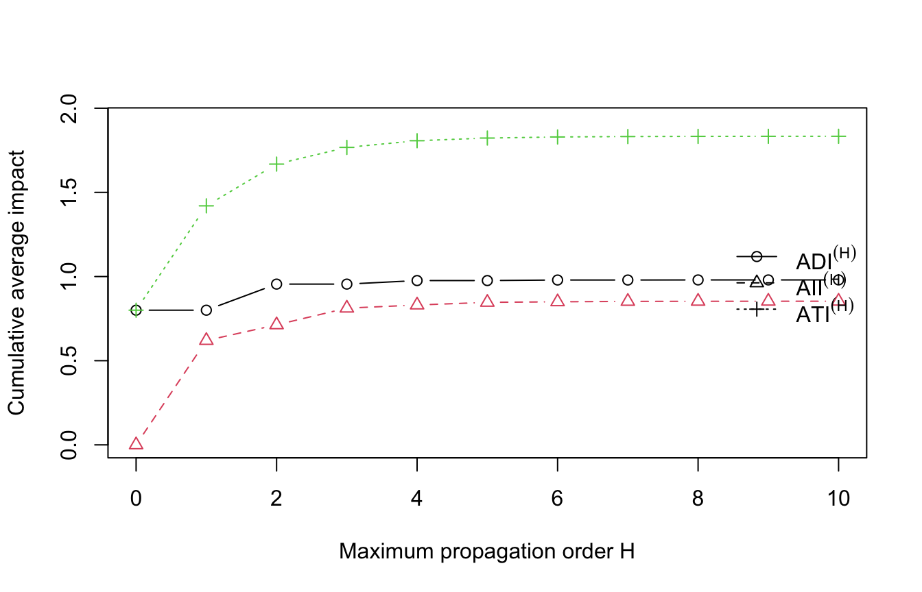
In this example, the total impact accumulates rapidly because the contribution of each additional order is multiplied by a further power of \(\rho\). The direct and indirect components need not converge at the same rate because the diagonal and off-diagonal elements of \(\mathbf{W}^{h}\) evolve differently across propagation orders.
2.4.6.10 Step 10: Visualize propagation from region 2
We now return to the one-unit increase in transport accessibility in region 2. Let \(\mathbf{e}_2\) denote the second unit vector. The vector \[ \mathbf{C}_h\mathbf{e}_2 \] shows the contribution of propagation order \(h\) to the outcomes in all four regions. Summing these vectors from order \(0\) through order \(H\) gives \[ \sum_{h=0}^{H}\mathbf{C}_h\mathbf{e}_2 = \mathbf{S}^{(H)}\mathbf{e}_2. \]
The following code calculates both the order-specific and cumulative regional responses.
shock_region_example <- 2
shock_example <- rep(0, n_example)
shock_example[shock_region_example] <- 1

shock_by_order_example <- do.call(
  rbind,
  lapply(
    impact_by_order_example,
    function(C_h) as.numeric(C_h %*% shock_example)
  )
)

colnames(shock_by_order_example) <- paste(
  "Region",
  seq_len(n_example)
)
rownames(shock_by_order_example) <- 0:H_max

shock_cumulative_example <- apply(
  shock_by_order_example,
  MARGIN = 2,
  FUN = cumsum
)

# Display the first six propagation orders.
round(shock_by_order_example[1:6, ], digits = 4)
Region 1 Region 2 Region 3 Region 4
0 0.0000 0.8000 0.0000 0.0000
1 0.6200 0.0000 0.3100 0.0000
2 0.0000 0.1860 0.0000 0.1240
3 0.0744 0.0000 0.0620 0.0000
4 0.0000 0.0273 0.0000 0.0248
5 0.0109 0.0000 0.0104 0.0000The cumulative response through order \(H=10\) can be compared with the exact second column of the complete impact matrix.
propagation_check_example <- data.frame(
  region = seq_len(n_example),
  cumulative_through_H = shock_cumulative_example[H_max + 1, ],
  complete_impact = S_example[, shock_region_example]
)

propagation_check_example$difference <-
  propagation_check_example$complete_impact -
  propagation_check_example$cumulative_through_H

propagation_check_display <- propagation_check_example
propagation_check_display[-1] <- round(
  propagation_check_display[-1],
  digits = 6
)

propagation_check_display
region cumulative_through_H complete_impact difference
Region 1 1 0.707290 0.707341 5.2e-05
Region 2 2 1.018333 1.018353 2.1e-05
Region 3 3 0.384373 0.384425 5.2e-05
Region 4 4 0.153749 0.153770 2.1e-05The following bubble plot makes the propagation sequence visible. Each column represents one power of \(\mathbf{W}\). The size and shading of a circle indicate the magnitude of the contribution received by a region at that order.
H_plot <- 5
shock_plot_example <- shock_by_order_example[1:(H_plot + 1), ]
shock_scale_example <- shock_plot_example / max(shock_plot_example)

plot(
  NA,
  xlim = c(-0.5, H_plot + 0.5),
  ylim = c(0.5, n_example + 0.5),
  xaxt = "n",
  yaxt = "n",
  xlab = "Propagation order h",
  ylab = "Region",
  xaxs = "i",
  yaxs = "i"
)

axis(1, at = 0:H_plot)
axis(2, at = seq_len(n_example), las = 1)
abline(v = 0:H_plot, h = seq_len(n_example), lty = 3)

for (h in 0:H_plot) {
  for (i in seq_len(n_example)) {

    relative_size <- shock_scale_example[h + 1, i]

    if (shock_plot_example[h + 1, i] > 0) {
      points(
        h,
        i,
        pch = 21,
        cex = 0.8 + 4 * sqrt(relative_size),
        bg = gray(0.95 - 0.45 * relative_size)
      )

      text(
        h,
        i,
        labels = sprintf(
          "%.3f",
          shock_plot_example[h + 1, i]
        ),
        cex = 0.65
      )
    }
  }
}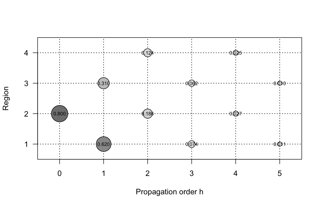
At order \(0\), only region 2 is affected. At order \(1\), the effect reaches regions 1 and 3, which are directly connected to region 2. At order \(2\), part of the effect returns to region 2 through spatial feedback, while another part reaches region 4. Subsequent orders contain progressively smaller contributions, including effects that revisit previously affected regions.
The index \(h\) should not be interpreted as calendar time. In this cross-sectional model, it indexes powers of the spatial weights matrix and therefore successive walk lengths in the comparative-static propagation mechanism.
NoteMain lesson
The coefficients \(\beta\), \(\gamma\), and \(\rho\) are not themselves the final marginal effects of the SDM. The economically relevant effects are obtained from the complete matrix
\[ \left( \mathbf{I}_n-\rho\mathbf{W} \right)^{-1} \left( \beta\mathbf{I}_n+\gamma\mathbf{W} \right). \]
The direct, indirect, and total effects summarize different parts of this matrix. The power-series decomposition additionally reveals how the final comparative-static response is assembled through successive spatial links and feedback paths.
2.4.7 Applied Case Study: Growth and International Technological Spillovers
This application is based on the spatially augmented Solow model developed by Ertur and Koch (2007). Its main advantage is that the spatial econometric specification is not introduced merely as a statistical correction. Instead, it is derived from an economic mechanism in which knowledge generated in one country can cross national borders and affect productivity elsewhere.
The discussion focuses on the part of the article that leads from the production model to the steady-state spatial Durbin model. The later extension to heterogeneous country-specific convergence speeds is mentioned at the end, but it is not derived here.
The application connects five elements:
- a production model with domestic and international knowledge externalities;
- a spatial multiplier for the international diffusion of technology;
- a steady-state income equation that has the form of an SDM;
- structural restrictions that can be tested empirically; and
- direct, indirect, and total elasticities implied by the estimated model.
2.4.7.1 Production and Spatial Technological Interdependence
Consider \(n\) countries indexed by \(i=1,\ldots,n\). Output in country \(i\) is produced according to \[ Y_i(t) = A_i(t) K_i(t)^{\alpha} L_i(t)^{1-\alpha}, \qquad 0<\alpha<1, \tag{2.77}\] where \(K_i(t)\) is physical capital, \(L_i(t)\) is labor, and \(A_i(t)\) is the country-specific level of technology.
Let \[ k_i(t) = \frac{K_i(t)}{L_i(t)} \] denote physical capital per worker. Technology is assumed to satisfy \[ A_i(t) = \Omega(t) k_i(t)^{\phi} \prod_{\substack{j=1 \\ j\neq i}}^{n} A_j(t)^{\eta w_{ij}}, \tag{2.78}\] where:
- \(\Omega(t)=\Omega_0e^{\mu t}\) is a common exogenous technology component, with constant growth rate \(\mu\);
- \(\phi\) measures the domestic knowledge externality generated by physical capital per worker;
- \(\eta\) measures the strength of international technological interdependence; and
- \(w_{ij}\) is an exogenous friction weight describing the relative technological connection from country \(j\) to country \(i\).
Following Ertur and Koch (2007), assume \(0\leq\phi<1\), \(0\leq\eta<1\), \(w_{ij}\geq0\), and \(w_{ii}=0\). The spatial weights matrix \(\mathbf{W}\) is row-standardized: \(\mathbf{W}\boldsymbol{\iota}_n=\boldsymbol{\iota}_n\).
The notation differs slightly from the original article. We retain \(\phi\) for the domestic capital externality but use \(\eta\) in place of the article’s \(\gamma\) for international technological interdependence. This avoids confusing the structural externality parameter with the coefficient vector \(\boldsymbol{\gamma}\) used earlier for spatially lagged explanatory variables.
Taking logarithms of Equation 2.78 gives \[ a_i(t) = \omega(t) + \phi k_i^{\ell}(t) + \eta \sum_{j=1}^{n} w_{ij}a_j(t), \] where \[ a_i(t)=\ln A_i(t), \qquad k_i^{\ell}(t)=\ln k_i(t), \qquad \omega(t)=\ln\Omega(t). \]
In matrix notation, \[ \mathbf{a}(t) = \omega(t)\boldsymbol{\iota}_n + \phi\mathbf{k}^{\ell}(t) + \eta\mathbf{W}\mathbf{a}(t). \tag{2.79}\]
Rearranging, \[ \left( \mathbf{I}_n-\eta\mathbf{W} \right) \mathbf{a}(t) = \omega(t)\boldsymbol{\iota}_n + \phi\mathbf{k}^{\ell}(t). \]
If \(\mathbf{I}_n-\eta\mathbf{W}\) is nonsingular, the technology vector is \[ \mathbf{a}(t) = \left( \mathbf{I}_n-\eta\mathbf{W} \right)^{-1} \left[ \omega(t)\boldsymbol{\iota}_n + \phi\mathbf{k}^{\ell}(t) \right]. \tag{2.80}\]
When \(|\eta|<1\), row stochasticity implies \(\varrho(\eta\mathbf{W})<1\), and the technology multiplier can be expanded as \[ \left( \mathbf{I}_n-\eta\mathbf{W} \right)^{-1} = \mathbf{I}_n + \eta\mathbf{W} + \eta^2\mathbf{W}^2 + \cdots. \]
The first term represents the contemporaneous domestic component. The higher-order terms describe propagation through paths of increasing length in the international network. As in the earlier discussion of the Neumann expansion, these powers are algebraic propagation orders, not calendar periods.
Proof. The production function per worker is \(y_i(t)=A_i(t)k_i(t)^{\alpha}\). Taking logarithms gives \(y_i^{\ell}(t)=a_i(t)+\alpha k_i^{\ell}(t)\). Stacking the observations, \[ \mathbf{y}^{\ell}(t) = \mathbf{a}(t) + \alpha\mathbf{k}^{\ell}(t). \]
Substitute Equation 2.80: \[ \begin{aligned} \mathbf{y}^{\ell}(t) &= \left( \mathbf{I}_n-\eta\mathbf{W} \right)^{-1} \left[ \omega(t)\boldsymbol{\iota}_n + \phi\mathbf{k}^{\ell}(t) \right] + \alpha\mathbf{k}^{\ell}(t) \\ &= \omega(t) \left( \mathbf{I}_n-\eta\mathbf{W} \right)^{-1} \boldsymbol{\iota}_n + \left[ \alpha\mathbf{I}_n + \phi \left( \mathbf{I}_n-\eta\mathbf{W} \right)^{-1} \right] \mathbf{k}^{\ell}(t). \end{aligned} \]
Since \(\mathbf{W}\) is row-stochastic, \(\mathbf{W}\boldsymbol{\iota}_n=\boldsymbol{\iota}_n\). Therefore, \[ \begin{aligned} \left( \mathbf{I}_n-\eta\mathbf{W} \right) \boldsymbol{\iota}_n &= \boldsymbol{\iota}_n - \eta\mathbf{W}\boldsymbol{\iota}_n \\ &= \left( 1-\eta \right) \boldsymbol{\iota}_n. \end{aligned} \]
Because \(|\eta|<1\), we have \(\eta\neq1\), and the inverse exists. Hence, \[ \left( \mathbf{I}_n-\eta\mathbf{W} \right)^{-1} \boldsymbol{\iota}_n = \frac{1}{1-\eta} \boldsymbol{\iota}_n. \]
Substituting this result proves Equation 2.81. Now differentiate Equation 2.81 with respect to \(k_j^{\ell}(t)\). Let \(\mathbf{e}_j\) be the \(j\)th column of \(\mathbf{I}_n\). Since \[ \frac{ \partial\mathbf{k}^{\ell}(t) }{ \partial k_j^{\ell}(t) } = \mathbf{e}_j, \] we obtain \[ \begin{aligned} \frac{ \partial\mathbf{y}^{\ell}(t) }{ \partial k_j^{\ell}(t) } &= \left[ \alpha\mathbf{I}_n + \phi \left( \mathbf{I}_n-\eta\mathbf{W} \right)^{-1} \right] \mathbf{e}_j. \end{aligned} \]
The \(i\)th element of this derivative is \[ \alpha\mathbf{1}\{i=j\} + \phi \left[ \left( \mathbf{I}_n-\eta\mathbf{W} \right)^{-1} \right]_{ij}, \] which proves Equation 2.82.
Finally, consider a proportional increase in capital per worker in every country. The vector of changes is proportional to \(\boldsymbol{\iota}_n\). The corresponding elasticity vector is \[ \begin{aligned} \left[ \alpha\mathbf{I}_n + \phi \left( \mathbf{I}_n-\eta\mathbf{W} \right)^{-1} \right] \boldsymbol{\iota}_n &= \alpha\boldsymbol{\iota}_n + \frac{\phi}{1-\eta} \boldsymbol{\iota}_n \\ &= \left( \alpha+\frac{\phi}{1-\eta} \right) \boldsymbol{\iota}_n. \end{aligned} \]
Thus, every country has the same social elasticity \(\alpha+\phi/(1-\eta)\) for a common proportional increase in capital.
The condition is the sufficient condition used by Ertur and Koch (2007) to ensure decreasing social returns to reproducible capital and local stability around the balanced growth path. It permits positive domestic and international externalities while ruling out an endogenous-growth outcome generated by those externalities.
2.4.7.2 From the Growth Model to a Spatial Durbin Model
Let \(s_i\) denote the saving rate, \(n_i\) the growth rate of labor, and \(\delta\) the depreciation rate. The common balanced-growth rate implied by exogenous technological progress is \[ g = \frac{ \mu }{ (1-\alpha)(1-\eta)-\phi }. \tag{2.85}\]
The denominator is positive under Equation 2.84. At the balanced-growth steady state of the Solow accumulation equation, \[ \frac{k_i^{*}}{y_i^{*}} = \frac{s_i}{n_i+g+\delta}. \]
Taking logarithms, \[ k_i^{\ell *} = y_i^{\ell *} + \ln s_i - \ln(n_i+g+\delta). \tag{2.86}\]
Define \[ S_i = \ln s_i - \ln(n_i+g+\delta) \] and let \(\mathbf{S}\) be the corresponding \(n\times1\) vector.
A useful intermediate representation of log output per worker is \[ \mathbf{y}^{\ell} = \omega\boldsymbol{\iota}_n + \left( \alpha+\phi \right) \mathbf{k}^{\ell} - \alpha\eta\mathbf{W}\mathbf{k}^{\ell} + \eta\mathbf{W}\mathbf{y}^{\ell}. \tag{2.87}\]
Substituting \(\mathbf{k}^{\ell *}=\mathbf{y}^{\ell *}+\mathbf{S}\) into Equation 2.87 gives \[ \begin{aligned} \mathbf{y}^{\ell *} = \omega\boldsymbol{\iota}_n + \left( \alpha+\phi \right) \left( \mathbf{y}^{\ell *}+\mathbf{S} \right) - \alpha\eta\mathbf{W} \left( \mathbf{y}^{\ell *}+\mathbf{S} \right) + \eta\mathbf{W}\mathbf{y}^{\ell *}. \end{aligned} \]
Expanding the right-hand side, \[ \begin{aligned} \mathbf{y}^{\ell *} = \omega\boldsymbol{\iota}_n + \left( \alpha+\phi \right) \mathbf{y}^{\ell *} + \left( \alpha+\phi \right) \mathbf{S} - \alpha\eta\mathbf{W}\mathbf{y}^{\ell *} - \alpha\eta\mathbf{W}\mathbf{S} + \eta\mathbf{W}\mathbf{y}^{\ell *}. \end{aligned} \]
Combining the two spatially lagged income terms, \[ -\alpha\eta\mathbf{W}\mathbf{y}^{\ell *} + \eta\mathbf{W}\mathbf{y}^{\ell *} = \eta \left( 1-\alpha \right) \mathbf{W}\mathbf{y}^{\ell *}. \]
Moving \((\alpha+\phi)\mathbf{y}^{\ell *}\) to the left-hand side gives \[ \begin{aligned} \left( 1-\alpha-\phi \right) \mathbf{y}^{\ell *} = \omega\boldsymbol{\iota}_n + \left( \alpha+\phi \right) \mathbf{S} - \alpha\eta\mathbf{W}\mathbf{S} + \eta \left( 1-\alpha \right) \mathbf{W}\mathbf{y}^{\ell *}. \end{aligned} \]
Assuming \(1-\alpha-\phi>0\), divide by this quantity and define \[ \beta = \frac{\alpha+\phi}{1-\alpha-\phi}, \tag{2.88}\]
\[ \gamma = -\frac{\alpha\eta}{1-\alpha-\phi}, \tag{2.89}\] and \[ \rho = \frac{\eta(1-\alpha)}{1-\alpha-\phi}. \tag{2.90}\]
The steady-state equation becomes \[ \mathbf{y}^{\ell *} = \beta_0\boldsymbol{\iota}_n + \beta\mathbf{S} + \gamma\mathbf{W}\mathbf{S} + \rho\mathbf{W}\mathbf{y}^{\ell *} + \boldsymbol{\varepsilon}, \tag{2.91}\]
To obtain an estimable cross-sectional equation, the initial technology term is written as a common intercept plus a country-specific disturbance. Accordingly, \(\beta_0\) absorbs the common component, while \(\boldsymbol{\varepsilon}\) captures country-specific differences in initial technology, resource endowments, climate, and other omitted determinants. This disturbance is introduced at the econometric stage; it is not part of the deterministic derivation above.
Expanding \(\mathbf{S}\), \[ \begin{aligned} \mathbf{y}^{\ell *} = \beta_0\boldsymbol{\iota}_n + \beta\ln\mathbf{s} - \beta\ln(\mathbf{n}+g+\delta) + \gamma\mathbf{W}\ln\mathbf{s} - \gamma\mathbf{W}\ln(\mathbf{n}+g+\delta) + \rho\mathbf{W}\mathbf{y}^{\ell *} + \boldsymbol{\varepsilon}. \end{aligned} \tag{2.92}\]
This is an SDM. The growth model therefore implies the joint coefficient restrictions \[ \beta_s=-\beta_n, \qquad \gamma_s=-\gamma_n. \tag{2.93}\]
The spatial lag of the constant is not included separately because, under row standardization, \(\mathbf{W}\boldsymbol{\iota}_n=\boldsymbol{\iota}_n\). It would therefore be perfectly collinear with the intercept.
2.4.7.3 Why Ordinary Least Squares Is Inconsistent
The SDM contains the endogenous spatial lag \(\mathbf{W}\mathbf{y}^{\ell *}\). Its endogeneity can be seen directly from the reduced form.
Proposition 2.10 (Endogeneity of the Spatially Lagged Dependent Variable) Suppose \[ \mathbb{E} \left( \boldsymbol{\varepsilon} \mid \mathbf{X},\mathbf{W} \right) = \mathbf{0} \] and \[ \mathbb{E} \left( \boldsymbol{\varepsilon} \boldsymbol{\varepsilon}^{\top} \mid \mathbf{X},\mathbf{W} \right) = \sigma^2\mathbf{I}_n. \] If \(\mathbf{I}_n-\rho\mathbf{W}\) is nonsingular, then, in general, \[ \mathbb{E} \left( \mathbf{W}\mathbf{y}^{\ell *} \boldsymbol{\varepsilon}^{\top} \mid \mathbf{X},\mathbf{W} \right) = \sigma^2 \mathbf{W} \left( \mathbf{I}_n-\rho\mathbf{W} \right)^{-1} \neq \mathbf{0}. \tag{2.94}\]
Moreover, \[ \mathbb{E} \left[ \left( \mathbf{W}\mathbf{y}^{\ell *} \right)^{\top} \boldsymbol{\varepsilon} \mid \mathbf{X},\mathbf{W} \right] = \sigma^2 \operatorname{tr} \left[ \mathbf{W} \left( \mathbf{I}_n-\rho\mathbf{W} \right)^{-1} \right], \tag{2.95}\] which is generally nonzero. Consequently, OLS applied directly to Equation 2.92 is generally inconsistent.
Proof. Write the SDM compactly as \[ \mathbf{y}^{\ell *} = \rho\mathbf{W}\mathbf{y}^{\ell *} + \mathbf{Z}\boldsymbol{\delta} + \boldsymbol{\varepsilon}, \] where \(\mathbf{Z}\) contains the intercept, the domestic regressors, and their spatial lags.
Rearranging, \[ \left( \mathbf{I}_n-\rho\mathbf{W} \right) \mathbf{y}^{\ell *} = \mathbf{Z}\boldsymbol{\delta} + \boldsymbol{\varepsilon}. \]
Premultiplying by the inverse gives \[ \mathbf{y}^{\ell *} = \left( \mathbf{I}_n-\rho\mathbf{W} \right)^{-1} \mathbf{Z}\boldsymbol{\delta} + \left( \mathbf{I}_n-\rho\mathbf{W} \right)^{-1} \boldsymbol{\varepsilon}. \]
Premultiplying by \(\mathbf{W}\), \[ \begin{aligned} \mathbf{W}\mathbf{y}^{\ell *} &= \mathbf{W} \left( \mathbf{I}_n-\rho\mathbf{W} \right)^{-1} \mathbf{Z}\boldsymbol{\delta} \\ &\quad+ \mathbf{W} \left( \mathbf{I}_n-\rho\mathbf{W} \right)^{-1} \boldsymbol{\varepsilon}. \end{aligned} \]
Multiply on the right by \(\boldsymbol{\varepsilon}^{\top}\) and take the conditional expectation: \[ \begin{aligned} \mathbb{E} \left( \mathbf{W}\mathbf{y}^{\ell *} \boldsymbol{\varepsilon}^{\top} \mid \mathbf{X},\mathbf{W} \right) &= \mathbf{W} \left( \mathbf{I}_n-\rho\mathbf{W} \right)^{-1} \mathbf{Z}\boldsymbol{\delta} \mathbb{E} \left( \boldsymbol{\varepsilon}^{\top} \mid \mathbf{X},\mathbf{W} \right) \\ &\quad+ \mathbf{W} \left( \mathbf{I}_n-\rho\mathbf{W} \right)^{-1} \mathbb{E} \left( \boldsymbol{\varepsilon} \boldsymbol{\varepsilon}^{\top} \mid \mathbf{X},\mathbf{W} \right). \end{aligned} \]
The first term is zero because the innovations have conditional mean zero. The second moment is \(\sigma^2\mathbf{I}_n\). Hence, \[ \begin{aligned} \mathbb{E} \left( \mathbf{W}\mathbf{y}^{\ell *} \boldsymbol{\varepsilon}^{\top} \mid \mathbf{X},\mathbf{W} \right) &= \sigma^2 \mathbf{W} \left( \mathbf{I}_n-\rho\mathbf{W} \right)^{-1}. \end{aligned} \]
This matrix is generally nonzero. The scalar normal-equation moment follows from the trace identity \[ \begin{aligned} \mathbb{E} \left[ \left( \mathbf{W}\mathbf{y}^{\ell *} \right)^{\top} \boldsymbol{\varepsilon} \mid \mathbf{X},\mathbf{W} \right] &= \operatorname{tr} \left\{ \mathbb{E} \left[ \boldsymbol{\varepsilon} \left( \mathbf{W}\mathbf{y}^{\ell *} \right)^{\top} \mid \mathbf{X},\mathbf{W} \right] \right\} \\ &= \operatorname{tr} \left\{ \mathbb{E} \left[ \mathbf{W}\mathbf{y}^{\ell *} \boldsymbol{\varepsilon}^{\top} \mid \mathbf{X},\mathbf{W} \right]^{\top} \right\} \\ &= \operatorname{tr} \left\{ \mathbb{E} \left[ \mathbf{W}\mathbf{y}^{\ell *} \boldsymbol{\varepsilon}^{\top} \mid \mathbf{X},\mathbf{W} \right] \right\} \\ &= \sigma^2 \operatorname{tr} \left[ \mathbf{W} \left( \mathbf{I}_n-\rho\mathbf{W} \right)^{-1} \right], \end{aligned} \]
Hence, the endogenous spatial lag generally violates the orthogonality condition required by OLS.
Ertur and Koch estimate the model by maximum likelihood, accounting for the Jacobian term \(\log|\mathbf{I}_n-\rho\mathbf{W}|\). Instrumental-variable and GMM estimators provide alternative approaches to the same simultaneity problem.
2.4.7.4 Data and Spatial Weights
The empirical application uses 91 countries over 1960–1995, corresponding to the non-oil sample used in the classic augmented Solow application and for which the required variables are available. The data come from Penn World Tables version 6.1. Real income per worker is measured using real GDP per worker, the saving rate is proxied by the average investment share of GDP, and \(n_i\) is the average growth rate of the working-age population.
The authors consider two distance-based spatial weights matrices. Before row standardization, their generic elements are \[ w_{ij}^{*(1)} = \begin{cases} 0, & i=j, \\ d_{ij}^{-2}, & i\neq j, \end{cases} \] and \[ w_{ij}^{*(2)} = \begin{cases} 0, & i=j, \\ \exp(-2d_{ij}), & i\neq j, \end{cases} \] where \(d_{ij}\) is the great-circle distance between national capitals.
The row-standardized weights are \[ w_{ij}^{(q)} = \frac{ w_{ij}^{*(q)} }{ \sum_{\ell=1}^{n} w_{i\ell}^{*(q)} }, \qquad q\in\{1,2\}. \]
The two matrices represent alternative assumptions about how quickly technological interaction decreases with geographic distance. Comparing results across them is therefore a substantive robustness exercise, not only a numerical sensitivity check.
2.4.7.5 Empirical Specification and Published Estimates
The unrestricted empirical SDM is \[ \begin{aligned} \ln\mathbf{y} = \beta_0\boldsymbol{\iota}_n + \beta_s\ln\mathbf{s} + \beta_n\ln(\mathbf{n}+0.05) + \gamma_s\mathbf{W}\ln\mathbf{s} + \gamma_n\mathbf{W}\ln(\mathbf{n}+0.05) + \rho\mathbf{W}\ln\mathbf{y} + \boldsymbol{\varepsilon}. \end{aligned} \tag{2.96}\]
The value \(g+\delta=0.05\) follows the conventional calibration used in the empirical growth literature.
The principal unrestricted estimates reported by Ertur and Koch (2007) are:
| Parameter | \(W_1\) | \(W_2\) |
|---|---|---|
| \(\widehat{\beta}_s\) | 0.825 | 0.792 |
| \(\widehat{\beta}_n\) | -1.498 | -1.451 |
| \(\widehat{\gamma}_s\) | -0.322 | -0.372 |
| \(\widehat{\gamma}_n\) | 0.571 | 0.137 |
| \(\widehat{\rho}\) | 0.740 | 0.658 |
The estimated spatial autoregressive coefficient is positive and statistically significant for both matrices. Likelihood-ratio tests do not reject the joint restrictions \(\beta_s=-\beta_n\) and \(\gamma_s=-\gamma_n\): the reported \(p\)-values are \(0.455\) for \(W_1\) and \(0.311\) for \(W_2\).
The restricted estimates used to recover the structural parameters are:
| Parameter | \(W_1\) | \(W_2\) |
|---|---|---|
| \(\widehat{\beta}\) | 0.841 | 0.818 |
| \(\widehat{\gamma}\) | -0.284 | -0.276 |
| \(\widehat{\rho}\) | 0.742 | 0.648 |
2.4.7.6 Recovering the Structural Parameters
The mappings in Equation 2.88, Equation 2.89, and Equation 2.90 can be inverted when international technological interdependence is nonzero.
Proposition 2.11 (Recovering the Growth Parameters) Suppose \(\beta\), \(\gamma\), and \(\rho\) satisfy Equation 2.88, Equation 2.89, and Equation 2.90, with \(\rho-\gamma\neq0\). Then \[ \alpha = \frac{-\gamma}{\rho-\gamma}, \tag{2.97}\]
\[ \eta = \frac{\rho-\gamma}{1+\beta}, \tag{2.98}\] and \[ \phi = \frac{\beta}{1+\beta} - \alpha. \tag{2.99}\]
Proof. Let \[ d = 1-\alpha-\phi. \]
From Equation 2.89 and Equation 2.90, \[ \begin{aligned} \rho-\gamma &= \frac{ \eta(1-\alpha) }{ d } - \left( -\frac{\alpha\eta}{d} \right) \\ &= \frac{ \eta(1-\alpha+\alpha) }{ d } \\ &= \frac{\eta}{d}. \end{aligned} \]
Because \(\rho-\gamma\neq0\), both \(\eta\) and the ratio above are nonzero. Dividing Equation 2.89 by this expression gives \[ \frac{\gamma}{\rho-\gamma} = \frac{ -\alpha\eta/d }{ \eta/d } = -\alpha. \]
Therefore, \[ \alpha = \frac{-\gamma}{\rho-\gamma}. \]
Next, Equation 2.88 implies \[ \beta = \frac{\alpha+\phi}{1-\alpha-\phi}. \]
Let \(q=\alpha+\phi\). Then \[ \beta = \frac{q}{1-q}. \]
Cross-multiplying, \[ \beta(1-q) = q. \]
Hence, \[ \beta = q(1+\beta), \] so \[ q = \alpha+\phi = \frac{\beta}{1+\beta}. \]
It follows that \[ \phi = \frac{\beta}{1+\beta} - \alpha. \]
Moreover, \[ d = 1-\alpha-\phi = 1- \frac{\beta}{1+\beta} = \frac{1}{1+\beta}. \]
Since \(\rho-\gamma=\eta/d\), \[ \eta = d(\rho-\gamma) = \frac{\rho-\gamma}{1+\beta}. \]
This proves the three recovery formulas.
NoteIdentification when technological interdependence is absent
If \(\eta=0\), then \(\rho=\gamma=0\). In that case, \(\beta\) identifies only the sum \(\alpha+\phi\), not \(\alpha\) and \(\phi\) separately. Thus, the condition \(\rho-\gamma\neq0\) is not merely algebraic: it is the condition that allows the private capital share and the domestic capital externality to be separately recovered from the spatial coefficients.
The following code reproduces the implied parameters.
# Store the restricted SDM estimates reported for the two spatial
# weights matrices.
restricted_growth_estimates <- data.frame(
  weights = c("W1", "W2"),
  beta = c(0.841, 0.818),
  gamma = c(-0.284, -0.276),
  rho = c(0.742, 0.648)
)

# Recover the structural production and externality parameters from
# the estimated SDM coefficients.
restricted_growth_estimates$alpha <- with(
  restricted_growth_estimates,
  -gamma / (rho - gamma)
)

restricted_growth_estimates$eta <- with(
  restricted_growth_estimates,
  (rho - gamma) / (1 + beta)
)

restricted_growth_estimates$phi <- with(
  restricted_growth_estimates,
  beta / (1 + beta) - alpha
)

# Calculate the total social elasticity of output with respect to a
# common proportional increase in capital.
restricted_growth_estimates$social_return <- with(
  restricted_growth_estimates,
  alpha + phi / (1 - eta)
)

# Round only the numeric columns.
numeric_columns <- vapply(
  restricted_growth_estimates,
  is.numeric,
  logical(1)
)

restricted_growth_estimates[numeric_columns] <- lapply(
  restricted_growth_estimates[numeric_columns],
  round,
  digits = 3
)

restricted_growth_estimates
weights beta gamma rho alpha eta phi social_return
1 W1 0.841 -0.284 0.742 0.277 0.557 0.180 0.683
2 W2 0.818 -0.276 0.648 0.299 0.508 0.151 0.606Using the rounded coefficient estimates reported in the article, the recovered values are approximately:
| Parameter | \(W_1\) | \(W_2\) |
|---|---|---|
| \(\widehat{\alpha}\) | 0.277 | 0.299 |
| \(\widehat{\phi}\) | 0.180 | 0.151 |
| \(\widehat{\eta}\) | 0.557 | 0.508 |
| \(\widehat{\alpha}+\widehat{\phi}/(1-\widehat{\eta})\) | 0.683 | 0.606 |
The estimated private capital share is close to one-third. Domestic capital externalities and international technological interdependence are positive, but the estimated social return remains below one. The empirical results are therefore consistent with decreasing social returns and conditional convergence rather than explosive endogenous growth.
2.4.7.7 Marginal Effects of Saving and Effective Depreciation
The coefficient estimates of an SDM are not the final elasticities. Let \[ \mathbf{B}(\rho) = \mathbf{I}_n-\rho\mathbf{W}. \]
The elasticity matrix for the saving rate is \[ \mathbf{S}_{s}(\rho) = \mathbf{B}(\rho)^{-1} \left( \beta_s\mathbf{I}_n + \gamma_s\mathbf{W} \right). \tag{2.100}\]
Because \(\mathbf{B}(\rho)^{-1}\) is a function of \(\mathbf{W}\), it commutes with \(\mathbf{W}\). Using \[ \mathbf{B}(\rho)^{-1} = \mathbf{I}_n + \rho\mathbf{W}\mathbf{B}(\rho)^{-1}, \] the same matrix can be written in the form used by Ertur and Koch (2007): \[ \mathbf{S}_{s}(\rho) = \beta_s\mathbf{I}_n + \left( \beta_s\rho+\gamma_s \right) \mathbf{W} \mathbf{B}(\rho)^{-1}. \tag{2.101}\]
Its \((i,j)\)th element is \[ \left[ \mathbf{S}_{s}(\rho) \right]_{ij} = \frac{ \partial\ln y_i }{ \partial\ln s_j }. \]
The elasticity matrix for effective depreciation is \[ \mathbf{S}_{n}(\rho) = \mathbf{B}(\rho)^{-1} \left( \beta_n\mathbf{I}_n + \gamma_n\mathbf{W} \right). \tag{2.102}\]
Under the theoretical restrictions, \[ \beta_n=-\beta_s \] and \[ \gamma_n=-\gamma_s. \]
Therefore, \[ \mathbf{S}_{n}(\rho) = -\mathbf{S}_{s}(\rho). \tag{2.103}\]
This symmetry is imposed by the theoretical Solow structure. It need not hold exactly in an unrestricted empirical SDM.
Because \(\mathbf{W}\) is row-stochastic, the average total elasticities have closed forms: \[ \operatorname{ATI}_{s} = \frac{ \beta_s+\gamma_s }{ 1-\rho } \tag{2.104}\] and \[ \operatorname{ATI}_{n} = \frac{ \beta_n+\gamma_n }{ 1-\rho }. \tag{2.105}\]
Using the unrestricted estimates gives:
| Matrix | Saving ATI | Effective-depreciation ATI |
|---|---|---|
| \(W_1\) | 1.935 | -3.565 |
| \(W_2\) | 1.228 | -3.842 |
These are average total elasticities. Because \(\mathbf{W}\) is row-stochastic, every row sum of the impact matrix is the same. Thus, under \(W_1\), a common one-percent increase in saving rates in all countries changes steady-state income per worker in each country by approximately \(1.935\) percent after all spatial feedback effects have occurred.
The article reports average saving elasticities of approximately \(0.90\) under \(W_1\) and \(0.84\) under \(W_2\), and average effective-depreciation elasticities of approximately \(-1.65\) and \(-1.69\). The article does not label these quantities using the later ADI–AII–ATI terminology. However, they cannot be row-sum total elasticities, because the published SDM coefficients and the row-stochastic formula imply the ATI values shown above. Since the discussion immediately preceding the reported averages distinguishes diagonal elasticities from off-diagonal cross-elasticities, the natural interpretation is that the reported averages are mean diagonal elasticities, that is, ADIs. Under that interpretation, the saving decomposition is:
| Matrix | Saving ADI | Saving AII | Saving ATI |
|---|---|---|---|
| \(W_1\) | 0.900 | 1.035 | 1.935 |
| \(W_2\) | 0.840 | 0.388 | 1.228 |
For effective depreciation, the corresponding reconstructed decomposition is:
| Matrix | Depreciation ADI | Depreciation AII | Depreciation ATI |
|---|---|---|---|
| \(W_1\) | -1.650 | -1.915 | -3.565 |
| \(W_2\) | -1.690 | -2.152 | -3.842 |
NoteReconstructed impact decomposition
The ATI values are calculated directly from the published unrestricted SDM coefficients and the row-stochastic formula. The ADI interpretation of the reported averages is an inference from the surrounding discussion and from their incompatibility with the row-sum totals implied by the published coefficients. The AII values are then obtained as ATI minus ADI. This decomposition is pedagogically useful, but it is not presented as a separate table in the original article.
The following code reproduces these calculations.
# Enter the unrestricted SDM coefficients and the average diagonal
# elasticities discussed in the article.
growth_impacts <- data.frame(
  weights = c("W1", "W2"),
  beta_s = c(0.825, 0.792),
  gamma_s = c(-0.322, -0.372),
  beta_n = c(-1.498, -1.451),
  gamma_n = c(0.571, 0.137),
  rho = c(0.740, 0.658),
  ADI_s = c(0.900, 0.840),
  ADI_n = c(-1.650, -1.690)
)

# Row standardization yields a closed-form average total impact.
growth_impacts$ATI_s <- with(
  growth_impacts,
  (beta_s + gamma_s) / (1 - rho)
)

growth_impacts$ATI_n <- with(
  growth_impacts,
  (beta_n + gamma_n) / (1 - rho)
)

# The average indirect impact is the difference between the average
# total and average direct impacts.
growth_impacts$AII_s <- with(
  growth_impacts,
  ATI_s - ADI_s
)

growth_impacts$AII_n <- with(
  growth_impacts,
  ATI_n - ADI_n
)

# Select and round the impact summaries without attempting to round
# the character column containing the matrix names.
growth_impact_summary <- growth_impacts[
  c(
    "weights",
    "ADI_s",
    "AII_s",
    "ATI_s",
    "ADI_n",
    "AII_n",
    "ATI_n"
  )
]

numeric_columns <- vapply(
  growth_impact_summary,
  is.numeric,
  logical(1)
)

growth_impact_summary[numeric_columns] <- lapply(
  growth_impact_summary[numeric_columns],
  round,
  digits = 3
)

growth_impact_summary
weights ADI_s AII_s ATI_s ADI_n AII_n ATI_n
1 W1 0.90 1.035 1.935 -1.65 -1.915 -3.565
2 W2 0.84 0.388 1.228 -1.69 -2.152 -3.842The negative estimate of \(\gamma_s\) does not imply that the final indirect effect of saving is negative. The final spillover effect depends on the entire matrix \[ \left( \mathbf{I}_n-\rho\mathbf{W} \right)^{-1} \left( \beta_s\mathbf{I}_n+\gamma_s\mathbf{W} \right), \] not on \(\gamma_s\) alone. In the published estimates, the positive feedback generated by \(\rho\) is sufficiently strong for the average indirect saving effect to be positive.
2.4.7.8 Testing the Economic Model
The theoretical model generates several empirically testable implications.
First, the domestic coefficients should satisfy \[ \beta_s+\beta_n=0. \]
Second, the contextual coefficients should satisfy \[ \gamma_s+\gamma_n=0. \]
Third, the absence of domestic capital externalities, \(\phi=0\), implies a common-factor restriction.
To see this, set \(\phi=0\) in the structural mappings. Then \[ \beta = \frac{\alpha}{1-\alpha}, \]
\[ \gamma = -\frac{\alpha\eta}{1-\alpha}, \] and \[ \rho = \eta. \]
Therefore, \[ \gamma = -\rho\beta. \tag{2.106}\]
In the expanded empirical equation, this implies \[ \gamma_s+\rho\beta_s=0, \qquad \gamma_n+\rho\beta_n=0. \tag{2.107}\]
Provided that the same \(\mathbf{W}\) is used and \(\mathbf{I}_n-\rho\mathbf{W}\) is nonsingular, the SDM then collapses to a spatial error representation. Testing the common-factor restriction is thus an economic test of whether the domestic capital externality is absent, not merely a mechanical model-selection exercise.
The evidence should be stated carefully. In the unrestricted specification, the reported likelihood-ratio \(p\)-values for the common-factor restrictions are \(0.052\) under \(W_1\) and \(0.121\) under \(W_2\). After imposing the Solow sign-symmetry restrictions, the corresponding \(p\)-values are \(0.010\) and \(0.054\). The evidence against \(\phi=0\) is therefore strongest for \(W_1\) and borderline for \(W_2\), although Ertur and Koch (2007) interpret the overall results as supporting positive domestic physical-capital externalities together with international technological interdependence.
2.4.7.9 What This Application Teaches
This application illustrates several general lessons.
A spatial econometric specification should ideally follow from a clearly defined interaction mechanism. Here, geographic links matter because technology and knowledge diffuse across countries.
The spatial weights matrix is part of the economic model. An inverse-square distance matrix and an exponential-distance matrix represent different rates of spatial decay and lead to different magnitudes of the estimated impacts.
The coefficient on a spatially lagged explanatory variable is not itself an indirect effect. The final effect depends jointly on \(\beta_r\), \(\gamma_r\), \(\rho\), and the complete structure of \(\mathbf{W}\).
Theoretical restrictions can be used to recover economically meaningful parameters such as the private capital share, domestic capital externalities, and international technological interdependence.
Finally, spatial dependence and spatial heterogeneity are distinct. The article later allows convergence parameters to vary locally across countries. That extension is important, but the central lesson for this chapter is already visible in the global SDM: countries cannot be treated as isolated observations when knowledge and growth spill across borders.
2.5 Chapter Summary
This chapter introduced the principal linear spatial econometric models and showed how their interpretations depend on the location of spatial dependence.
The SLM and SAC contain endogenous interaction through \(\mathbf{W}\mathbf{y}\). The SEM and SDEM place spatial dependence in the disturbance process. The SLX and SDM include contextual effects through \(\mathbf{W}\mathbf{X}\), while the GNS nests all three channels.
The reduced form of a spatial autoregressive model contains the multiplier \[ \left( \mathbf{I}_n-\rho\mathbf{W} \right)^{-1}. \]
This inverse exists only for admissible values of \(\rho\). The Neumann-series representation additionally requires \(|\rho|\varrho(\mathbf{W})<1\).
In models with an endogenous spatial lag, regression coefficients are not marginal effects. The impact matrix for explanatory variable \(r\) in the SDM is \[ \mathbf{S}_r(\rho) = \left( \mathbf{I}_n-\rho\mathbf{W} \right)^{-1} \left( \beta_r\mathbf{I}_n+\gamma_r\mathbf{W} \right). \]
Its diagonal elements are direct effects, its off-diagonal elements are indirect effects, its row sums measure effects arriving at each unit, and its column sums measure effects originating from each unit.
Average direct, indirect, and total impacts provide compact summaries, but regional spill-in and spill-out effects may differ substantially across locations.
The growth application demonstrated how an economic model of technological interdependence can generate an SDM, impose testable coefficient restrictions, identify structural parameters, and produce economically meaningful elasticities.
2.6 Exercises
Exercise 2.1 (Classifying Spatial Models) For each specification below, identify the model and state whether spatial dependence enters through the dependent variable, explanatory variables, or disturbances.
\[ \mathbf{y} = \mathbf{X}\boldsymbol{\beta} + \mathbf{W}\mathbf{X}\boldsymbol{\gamma} + \boldsymbol{\varepsilon}. \]
\[ \begin{aligned} \mathbf{y} &= \rho\mathbf{W}\mathbf{y} + \mathbf{X}\boldsymbol{\beta} + \mathbf{u}, \\ \mathbf{u} &= \lambda\mathbf{W}\mathbf{u} + \boldsymbol{\varepsilon}. \end{aligned} \]
\[ \begin{aligned} \mathbf{y} &= \mathbf{X}\boldsymbol{\beta} + \mathbf{W}\mathbf{X}\boldsymbol{\gamma} + \mathbf{u}, \\ \mathbf{u} &= \lambda\mathbf{W}\mathbf{u} + \boldsymbol{\varepsilon}. \end{aligned} \]
\[ \mathbf{y} = \rho\mathbf{W}\mathbf{y} + \mathbf{X}\boldsymbol{\beta} + \mathbf{W}\mathbf{X}\boldsymbol{\gamma} + \boldsymbol{\varepsilon}. \]
Exercise 2.2 (Deriving a Reduced Form) Consider
\[ \mathbf{y} = \rho\mathbf{W}\mathbf{y} + \mathbf{X}\boldsymbol{\beta} + \boldsymbol{\varepsilon}. \]
- Derive the reduced form.
- Derive the conditional mean.
- If \(\operatorname{Var}(\boldsymbol{\varepsilon}\mid\mathbf{X},\mathbf{W}) =\sigma^2\mathbf{I}_n\), derive the conditional variance of \(\mathbf{y}\).
- Explain why the conditional variance is generally non-diagonal even when the innovations are uncorrelated.
Exercise 2.3 (Spectral Bounds) Let the eigenvalues of \(\mathbf{W}\) be
\[ 1, \qquad 0.5, \qquad -0.4, \qquad -0.8. \]
- Determine the spectral radius.
- Give the sufficient symmetric interval based on the spectral radius.
- Give the largest open real-eigenvalue interval containing zero.
- Determine whether each value is admissible: \(\rho=0.9\), \(\rho=-1.1\), \(\rho=1\), and \(\rho=-1.3\).
- Explain why the two intervals obtained in parts 2 and 3 differ.
Exercise 2.4 (Neumann Expansion) Suppose \(|\rho|\varrho(\mathbf{W})<1\).
Prove the finite matrix identity
\[ \left( \mathbf{I}_n-\rho\mathbf{W} \right) \sum_{h=0}^{H} \rho^h\mathbf{W}^h = \mathbf{I}_n-\rho^{H+1}\mathbf{W}^{H+1}. \]
State the additional limit required to obtain the infinite expansion.
Explain why nonsingularity alone is insufficient.
Construct a scalar counterexample.
Exercise 2.5 (Rows, Columns, and Spatial Direction) Let
\[ \mathbf{S}_r = \begin{pmatrix} 0.9 & 0.3 & 0.1 \\ 0.2 & 1.0 & 0.4 \\ 0.1 & 0.2 & 0.8 \end{pmatrix}. \]
- Calculate the direct effect for every region.
- Calculate the spill-in effect for every region.
- Calculate the spill-out effect for every region.
- Calculate total-to and total-from effects.
- Verify that average spill-in equals average spill-out.
- Explain why the region-specific spill-in and spill-out effects need not be equal.
Exercise 2.6 (Average Impact Measures) Using the matrix in Exercise 2.5:
- Calculate ADI.
- Calculate ATI as the average of the row sums.
- Calculate ATI as the average of the column sums.
- Calculate AII.
- Calculate the arithmetic mean of all nine matrix elements.
- Explain why the answer to part 5 differs from ATI.
Exercise 2.7 (Reproducing the Four-Region Example) Reproduce the transport-accessibility example in Section 2.4.6.
- Construct the matrix \(\mathbf{W}\) in R.
- Verify that it is row-stochastic but not symmetric.
- Calculate \(\mathbf{B}(\rho)=\mathbf{I}_4-\rho\mathbf{W}\).
- Calculate the complete impact matrix.
- Reproduce the direct, spill-in, spill-out, total-to, and total-from effects.
- Change \(\rho\) from \(0.4\) to \(0.7\). Explain how the impact measures change.
- Change \(\gamma\) from \(0.3\) to \(-0.3\). Determine whether the final average indirect effect must be negative.
Exercise 2.8 (Closed-Form Total Effect) Suppose \(\mathbf{W}\) is row-stochastic and
\[ \mathbf{S}_r(\rho) = \left( \mathbf{I}_n-\rho\mathbf{W} \right)^{-1} \left( \beta_r\mathbf{I}_n+\gamma_r\mathbf{W} \right). \]
Prove that
\[ \operatorname{ATI}_r = \frac{\beta_r+\gamma_r}{1-\rho}. \]
State every property of \(\mathbf{W}\) used in the proof.
Exercise 2.9 (Technology Multiplier) Consider the technology equation
\[ \mathbf{a} = \omega\boldsymbol{\iota}_n + \phi\mathbf{k}^{\ell} + \eta\mathbf{W}\mathbf{a}. \]
- Derive its reduced form.
- Expand the reduced form as a Neumann series.
- Interpret the terms involving \(\mathbf{W}\), \(\mathbf{W}^2\), and \(\mathbf{W}^3\).
- Show that a common increase in log capital has social elasticity \(\alpha+\phi/(1-\eta)\).
- Explain the economic meaning of the condition \(\alpha+\phi/(1-\eta)<1\).
Exercise 2.10 (Deriving the Growth SDM) Start from Equation 2.87 and the steady-state relation
\[ \mathbf{k}^{\ell *} = \mathbf{y}^{\ell *} + \ln\mathbf{s} - \ln(\mathbf{n}+g+\delta). \]
Derive Equation 2.92 without skipping algebraic steps. Identify:
- the coefficient on domestic saving;
- the coefficient on domestic effective depreciation;
- the coefficient on spatially lagged saving;
- the coefficient on spatially lagged effective depreciation; and
- the spatial autoregressive coefficient.
Verify the restrictions in Equation 2.93.
Exercise 2.11 (Recovering Structural Growth Parameters) Using the restricted estimates for \(W_1\),
\[ \widehat{\beta}=0.841, \qquad \widehat{\gamma}=-0.284, \qquad \widehat{\rho}=0.742, \]
calculate:
- \(\widehat{\alpha}\);
- \(\widehat{\eta}\);
- \(\widehat{\phi}\); and
- the social return \(\widehat{\alpha}+\widehat{\phi}/(1-\widehat{\eta})\).
Determine whether the estimated model satisfies decreasing social returns.
Exercise 2.12 (Capital Externalities and the Common Factor) Using the structural mappings for the growth model:
- impose \(\phi=0\);
- show that \(\rho=\eta\);
- show that \(\gamma=-\rho\beta\);
- explain why this is a common-factor restriction; and
- explain why rejecting this restriction provides evidence of domestic physical-capital externalities.
Exercise 2.13 (Impacts from Published Estimates) For \(W_1\), use
\[ \widehat{\beta}_s=0.825, \qquad \widehat{\gamma}_s=-0.322, \qquad \widehat{\rho}=0.740. \]
- Calculate the saving ATI.
- Given an ADI of \(0.900\), calculate the AII.
- Explain why the negative value of \(\widehat{\gamma}_s\) does not imply a negative AII.
- Repeat the calculation for \(W_2\) using the estimates reported in
- Discuss why the two spatial weights matrices produce different impact estimates.
Exercise 2.14 (Endogeneity of the Spatial Lag) Starting from the reduced form of the SDM:
- derive \(\mathbb{E}( \mathbf{W}\mathbf{y}\boldsymbol{\varepsilon}^{\top} \mid\mathbf{X},\mathbf{W})\);
- explain why OLS is inconsistent;
- identify variables that could serve as instruments for \(\mathbf{W}\mathbf{y}\); and
- explain why spatial lags of exogenous regressors may be relevant instruments.
Exercise 2.15 (Alternative Spatial Weights) Suppose technological spillovers are represented by either inverse-square distance weights or exponential-distance weights.
- Explain the economic interpretation of each decay function.
- Describe how you would row-standardize each matrix.
- Explain why the diagonal should be set to zero.
- Discuss whether great-circle distance is plausibly exogenous.
- Propose one alternative measure of technological proximity and discuss why it could be endogenous.
- Explain why robustness to alternative matrices does not establish that either matrix is correctly specified.
Exercise 2.16 (Convergence and Half-Life) The spatial growth application reports convergence speeds of approximately \(0.017\) and \(0.015\) per year.
Show that the half-life associated with convergence speed \(\lambda\) is
\[ h = \frac{\ln 2}{\lambda}. \]
Calculate the half-life for each reported convergence speed.
Interpret the result economically.
Explain why heterogeneous convergence speeds may be more plausible than a single common speed across all countries.
Exercise 2.17 (Empirical Extension) Design an empirical application of an SDM in which the spatial interaction mechanism follows from economic theory.
Your proposal should specify:
- the dependent variable;
- the domestic explanatory variables;
- the mechanism generating \(\mathbf{W}\mathbf{y}\) or \(\mathbf{W}\mathbf{X}\);
- the construction of \(\mathbf{W}\);
- the expected signs of the coefficients;
- at least one theoretically motivated parameter restriction;
- the direct, indirect, and total effects of primary interest; and
- a robustness strategy using at least one alternative spatial weights matrix.
Appendix: Matrix Norms
This appendix collects the matrix norms and inequalities used repeatedly in the chapter.
2.6.1 Vector and Matrix Norms
Definition 2.6 (Vector norm) A vector norm on \(\mathbb R^n\) is a function \(\|\cdot\|\) satisfying, for every \(\mathbf x,\mathbf y\in\mathbb R^n\) and every scalar \(c\),
- \(\|\mathbf x\|\geq0\), with equality if and only if \(\mathbf x=\mathbf0\);
- \(\|c\mathbf x\|=|c|\,\|\mathbf x\|\);
- \(\|\mathbf x+\mathbf y\|\leq\|\mathbf x\|+\|\mathbf y\|\).
Let \(\mathbf x = (x_1, \ldots, x_n)^\top\). The most common vector norms are the sum norm \[\|\mathbf x\|_1 = \sum_{i=1}^{n}|x_i|, \] the euclidean norm \[\|\mathbf x\|_2 = \left( \sum_{i=1}^{n}x_i^2 \right)^{1/2}, \] and the max norm \[\|\mathbf x\|_{\infty} = \max_{1\leq i\leq n}|x_i|. \]
Definition 2.7 (Matrix norm) A matrix norm is a function \(\|\cdot\|\) satisfying, for conformable matrices \(\mathbf A\) and \(\mathbf B\) and every scalar \(c\),
- \(\|\mathbf A\|\geq0\), with equality if and only if \(\mathbf A=\mathbf0\);
- \(\|c\mathbf A\|=|c|\,\|\mathbf A\|\);
- \(\|\mathbf A+\mathbf B\|\leq \|\mathbf A\|+\|\mathbf B\|\).
A matrix norm is submultiplicative if it also satisfies \[\|\mathbf A\mathbf B\| \leq \|\mathbf A\|\,\|\mathbf B\|.\]
The distinction matters because positivity, homogeneity, and the triangle inequality define a norm, whereas submultiplicativity is an additional property. All induced matrix norms defined below are submultiplicative.
Definition 2.8 (Induced matrix norm) Given a vector norm \(\|\cdot\|_p\), the corresponding induced matrix norm is \[\|\mathbf A\|_p = \sup_{\mathbf x\neq\mathbf0} \frac{ \|\mathbf A\mathbf x\|_p }{ \|\mathbf x\|_p }.\]
The induced \(1\)-norm is the maximum absolute column sum: \[\|\mathbf A\|_1 = \max_{1\leq j\leq n} \sum_{i=1}^{m}|a_{ij}|. \tag{2.108}\]
The induced infinity norm is the maximum absolute row sum: \[\|\mathbf A\|_{\infty} = \max_{1\leq i\leq m} \sum_{j=1}^{n}|a_{ij}|. \tag{2.109}\]
The induced Euclidean norm, also called the spectral norm, is \[\|\mathbf A\|_2 = \sqrt{ \lambda_{\max} \left( \mathbf A^{\top}\mathbf A \right) }, \tag{2.110}\] where \(\lambda_{\max}(\mathbf A^{\top}\mathbf A)\) is the largest eigenvalue of the symmetric positive-semidefinite matrix \(\mathbf A^{\top}\mathbf A\). Equivalently, \(\|\mathbf A\|_2\) is the largest singular value of \(\mathbf A\).
The Frobenius norm is \[\|\mathbf A\|_F = \left( \sum_{i=1}^{m} \sum_{j=1}^{n}a_{ij}^2 \right)^{1/2} = \sqrt{ \operatorname{tr} \left( \mathbf A^{\top}\mathbf A \right) }. \tag{2.111}\]
The Frobenius norm is submultiplicative, but it is not the matrix norm induced by the Euclidean vector norm. The latter is the spectral norm.
Proposition 2.12 (Formulas for the induced \(1\)- and infinity norms) For every \(m\times n\) matrix \(\mathbf A\), \[\|\mathbf A\|_1 = \max_j\sum_i|a_{ij}|\] and \[\|\mathbf A\|_{\infty} = \max_i\sum_j|a_{ij}|.\]
Proof. We first prove the formula for the induced \(1\)-norm. For any \(\mathbf x\in\mathbb R^n\), \[\begin{aligned} \|\mathbf A\mathbf x\|_1 &= \sum_{i=1}^{m} \left| \sum_{j=1}^{n}a_{ij}x_j \right| \\ &\leq \sum_{i=1}^{m} \sum_{j=1}^{n}|a_{ij}|\,|x_j| \\ &= \sum_{j=1}^{n} \left( \sum_{i=1}^{m}|a_{ij}| \right) |x_j| \\ &\leq \left[ \max_j \sum_{i=1}^{m}|a_{ij}| \right] \sum_{j=1}^{n}|x_j|. \end{aligned}\]
Therefore, \[\frac{\|\mathbf A\mathbf x\|_1}{\|\mathbf x\|_1} \leq \max_j\sum_i|a_{ij}|\] for every nonzero \(\mathbf x\). Taking the supremum gives \[\|\mathbf A\|_1 \leq \max_j\sum_i|a_{ij}|.\]
Let \(j^{*}\) be a column attaining the maximum, and choose \(\mathbf x=\mathbf e_{j^{*}}\), the corresponding coordinate vector. Then \(\|\mathbf x\|_1=1\) and \[\|\mathbf A\mathbf e_{j^{*}}\|_1 = \sum_i|a_{ij^{*}}|.\]
Thus the upper bound is attained, proving Equation 2.108.
For the infinity norm, let \(i^{*}\) be a row attaining the maximum absolute row sum. For any \(\mathbf x\), \[\begin{aligned} \|\mathbf A\mathbf x\|_{\infty} &= \max_i \left| \sum_j a_{ij}x_j \right| \\ &\leq \max_i \sum_j|a_{ij}|\,|x_j| \\ &\leq \left( \max_i\sum_j|a_{ij}| \right) \|\mathbf x\|_{\infty}. \end{aligned}\]
Hence \[\|\mathbf A\|_{\infty} \leq \max_i\sum_j|a_{ij}|.\]
To attain the bound, choose a vector satisfying \[x_j = \begin{cases} 1, & a_{i^{*}j}\geq0,\\ -1, & a_{i^{*}j}<0. \end{cases}\]
Then \(\|\mathbf x\|_{\infty}=1\) and \[(\mathbf A\mathbf x)_{i^{*}} = \sum_j|a_{i^{*}j}|.\]
Therefore, \[\|\mathbf A\mathbf x\|_{\infty} \geq \sum_j|a_{i^{*}j}|,\] which proves Equation 2.109.